


















Lesson 24 of 46 · Continuous Models with ODEs
SIR epidemics and predator-prey systems
Build coupled ODE models: the SIR epidemic with its reproduction number R0, and Lotka-Volterra predator-prey cycles, solved with a hand-written Runge-Kutta method.
Real systems have several parts that influence each other. Infected people create new infections and also recover. Foxes eat rabbits and so help themselves; fewer rabbits then means fewer foxes. To model this you write one equation for each quantity and let the equations share variables. A set of ODEs like this is a system. In this lesson you will build two classic systems, find the numbers that decide their behaviour, and meet a better solver than Euler's method.
What you will learn
- How to write the SIR model and interpret
β,γand the reproduction numberR₀. - How to compute the epidemic peak and final size from formulas and check them numerically.
- How the Lotka-Volterra equations produce cycles and what a phase plane shows.
- How the Runge-Kutta method (RK4) improves on Euler.
Key terms
SIR model: a compartment model splitting a population into Susceptible, Infected and Recovered people.
Basic reproduction number R₀: the average number of people one infected person infects in a fully susceptible population: R₀ = β/γ.
Phase plane: a plot of one state variable against another, with time left implicit.
RK4: the classical fourth-order Runge-Kutta method, which averages four slopes per step.
The SIR model
William Kermack and Anderson McKendrick published this model in 1927. Let S, I and R be the fractions of the population that are susceptible, infected and recovered (so S + I + R = 1). Two ideas drive the model:
- Infections happen when a susceptible person meets an infected one, at rate
β·S·I(β is the infection rate per day). - Infected people recover at rate
γ·I(γ is the recovery rate; the average infectious period is1/γdays).
dS/dt = −β·S·I
dI/dt = β·S·I − γ·I
dR/dt = γ·I
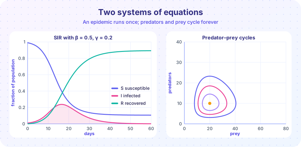
The three equations add up to zero, which is why the total stays fixed. The infection grows only while dI/dt > 0, that is when β·S > γ, or S > γ/β. At the start S ≈ 1, so an epidemic takes off exactly when R₀ = β/γ > 1. Taking β = 0.5 and γ = 0.2 per day gives R₀ = 2.5.
Two exact results come from dividing the equations:
- Peak. The infection peaks when
S = 1/R₀, andI_max = I₀ + S₀ − (1/R₀)·(1 + ln(R₀·S₀)). - Final size. The epidemic ends with
S∞satisfyingS∞ = S₀ · exp(−R₀·(1 − S∞)). Many people are never infected, but the epidemic ends because the pool of susceptibles falls below1/R₀, not because everyone caught it.
Notice the lesson for public health: vaccinating a fraction 1 − 1/R₀ of people means S starts below the threshold and the outbreak cannot grow. For R₀ = 2.5 that is 60 percent.
Runge-Kutta: four slopes are better than one
Euler uses the slope at the start of the step. RK4 samples the slope four times and takes a weighted average:
k1 = f(t, y)
k2 = f(t + h/2, y + h/2 · k1)
k3 = f(t + h/2, y + h/2 · k2)
k4 = f(t + h,   y + h · k3)
y_new = y + h/6 · (k1 + 2·k2 + 2·k3 + k4)
The error per whole run shrinks like h⁴: halve the step and the error drops by about 16. It costs four evaluations of f per step, but you can use a much larger h, so it usually wins. SciPy's solve_ivp uses a related adaptive Runge-Kutta pair by default.
Press Run (or Ctrl + Enter) to see the result here.
Program input · what you'd type while the program runs
Type the answers before you press Run, one per line. Each time the program reads a line (with input()), it gets the next line from this box.
Common misconceptions
"An epidemic ends when everyone has been infected." It ends when S falls below γ/β. In the simulation above roughly a tenth of the population is still susceptible at the end.
"R₀ is a property of the disease alone." It also depends on behaviour, density and contact patterns, because β includes how often people meet.
"A model that fits the early data predicts the peak." Early growth tells you β − γ, not β and γ separately. Different pairs give very different peaks. You will see this in the projects chapter.
Predator and prey
Alfred Lotka (1925) and Vito Volterra (1926) independently proposed a model of rabbits x and foxes y:
dx/dt = a·x − b·x·y
dy/dt = −c·y + d·x·y
Without foxes, rabbits grow exponentially at rate a. Each rabbit-fox meeting removes rabbits (b·x·y) and feeds foxes (d·x·y). Without rabbits, foxes die out at rate c. Setting both right-hand sides to zero gives a non-trivial equilibrium at x* = c/d and y* = a/b. With a = 1, b = 0.1, c = 1.5, d = 0.075 that is 20 prey and 10 predators.
Near the equilibrium the solutions do not settle down. They circle it forever, because the quantity V = d·x − c·ln(x) + b·y − a·ln(y) stays constant along every solution. Each initial condition gives its own closed loop in the phase plane. The prey peak first, then the predators, then the prey crash, then the predators crash: a lagged cycle.
Real ecosystems are less tidy (the model has no carrying capacity, for instance), but the lagged cycles of the snowshoe hare and the Canada lynx, recorded in fur-trading records for about ninety years, show the same qualitative rhythm.
Because V is constant, it is an excellent test of a numerical method: a good solver keeps V nearly constant, and a poor one lets it drift.
Press Run (or Ctrl + Enter) to see the result here.
Program input · what you'd type while the program runs
Type the answers before you press Run, one per line. Each time the program reads a line (with input()), it gets the next line from this box.
Explore the epidemic
Change β and γ. Watch R₀ cross 1: below it nothing happens, above it the infection curve rises and the peak grows quickly.
Check your understanding
Quick check · 5 questions
of 5 answered You scored / 5 · perfect!
-
1. In the SIR model with beta = 0.6 and gamma = 0.3 per day, what is R0?
R0 = beta / gamma = 0.6 / 0.3 = 2. -
2. When does the number of infected people start to grow in an SIR model?
dI/dt = (beta S - gamma) I is positive exactly when beta S > gamma, i.e. S > gamma/beta. -
3. R0 = 2.5. What fraction of the population must be immune to prevent an outbreak?
The threshold is 1 - 1/R0 = 1 - 0.4 = 0.6. -
4. In the Lotka-Volterra model, where is the non-trivial equilibrium?
Setting both derivatives to zero gives x = c/d (prey) and y = a/b (predators). -
5. By roughly what factor does RK4 reduce its error when the step size is halved?
RK4 is fourth order, so the error scales like h^4 and halving h divides it by 2^4 = 16.
Summary
- SIR:
dS/dt = −βSI,dI/dt = βSI − γI,dR/dt = γI; an epidemic needsR₀ = β/γ > 1. - The peak occurs at
S = 1/R₀; the final size solvesS∞ = S₀·e^(−R₀(1−S∞)). - Lotka-Volterra systems have an equilibrium
(c/d, a/b)surrounded by closed loops. - RK4 combines four slopes per step and has error of order
h⁴; Euler drifts off conserved loops.
Next: Chapter 5 review
Track your progress
Create a free account to tick off lessons and pick up where you left off on any device.
of Mathematical Modelling lessons completed