


















Lesson 18 of 46 · Discrete Dynamical Models
The Logistic Map and Chaos
Explore the logistic map x(n+1) = r x(n)(1 - x(n)): fixed points, stability, cobweb diagrams, the bifurcation diagram and sensitive dependence, with live simulations.
Is it possible for a rule as simple as "multiply a number by a constant and by one minus itself" to produce behavior so complicated that long-term prediction is impossible? Yes. In 1976 the biologist Robert May published a short, famous paper showing exactly that for a model of insect populations. The same equation became a doorway into the modern study of chaos.
This lesson walks through that doorway slowly, using only algebra and code.
What you will learn
- How the logistic map models crowding and where its equilibria are
- How to test stability with the derivative, and how to read a cobweb diagram
- How period doubling leads to chaos in the bifurcation diagram
- What sensitive dependence on initial conditions means in practice
Key terms
Logistic map: the rule xₙ₊₁ = r xₙ (1 − xₙ), where xₙ is the population as a fraction of the maximum (0 ≤ x ≤ 1).
Cobweb diagram: a picture of iteration between the curve y = f(x) and the line y = x.
Period-k cycle: a sequence of k values that repeats forever.
Bifurcation: a change in the long-run behavior as a parameter passes a critical value.
Chaos: bounded, deterministic behavior that never repeats and is extremely sensitive to the starting value.
From growth to crowding
Pure growth xₙ₊₁ = r xₙ explodes. Real populations run out of food and space. A neat fix: multiply growth by a factor that shrinks as the population nears its maximum. If x is the fraction of the maximum, the factor (1 − x) is 1 when the habitat is empty and 0 when it is full:
xₙ₊₁ = r xₙ (1 − xₙ), with 0 < r ≤ 4
The limit r ≤ 4 keeps x between 0 and 1 (the highest value of x(1 − x) is 1/4). The continuous version of this idea was written down by Pierre-François Verhulst in 1838; the discrete version is the logistic map.
Equilibria and stability
Solve x = r x (1 − x):
x* = 0(extinction), always an equilibrium.x* = 1 − 1/r, a positive equilibrium whenr > 1.
Stability of a fixed point of xₙ₊₁ = f(xₙ) depends on the slope there. A small deviation δ from x* becomes about f′(x*) · δ after one step, so it shrinks if |f′(x*)| < 1. Here f′(x) = r (1 − 2x):
- At
x* = 0:f′ = r, stable only forr < 1. - At
x* = 1 − 1/r:f′ = 2 − r, so|2 − r| < 1means1 < r < 3.
So up to r = 3 the population settles to a steady value. At r = 3 the slope reaches −1 and the fixed point loses stability. What happens next is the interesting part.
Cobweb diagrams
To see the iteration geometrically, draw the curve y = f(x) and the diagonal y = x. Start at x₀ on the horizontal axis, go up to the curve (that gives x₁ = f(x₀)), go across to the diagonal (so x₁ becomes the new input), then up again. The path spirals into a stable fixed point, or around a cycle.
Press Run (or Ctrl + Enter) to see the result here.
Program input · what you'd type while the program runs
Type the answers before you press Run, one per line. Each time the program reads a line (with input()), it gets the next line from this box.
With r = 2.8 the path spirals into the fixed point near 0.643; with r = 3.3 it settles onto a loop that visits two values; with r = 3.9 it wanders without settling.
The bifurcation diagram
To see all the long-run behaviors at once, plot for each r the values the sequence visits after a long transient. This is the bifurcation diagram.
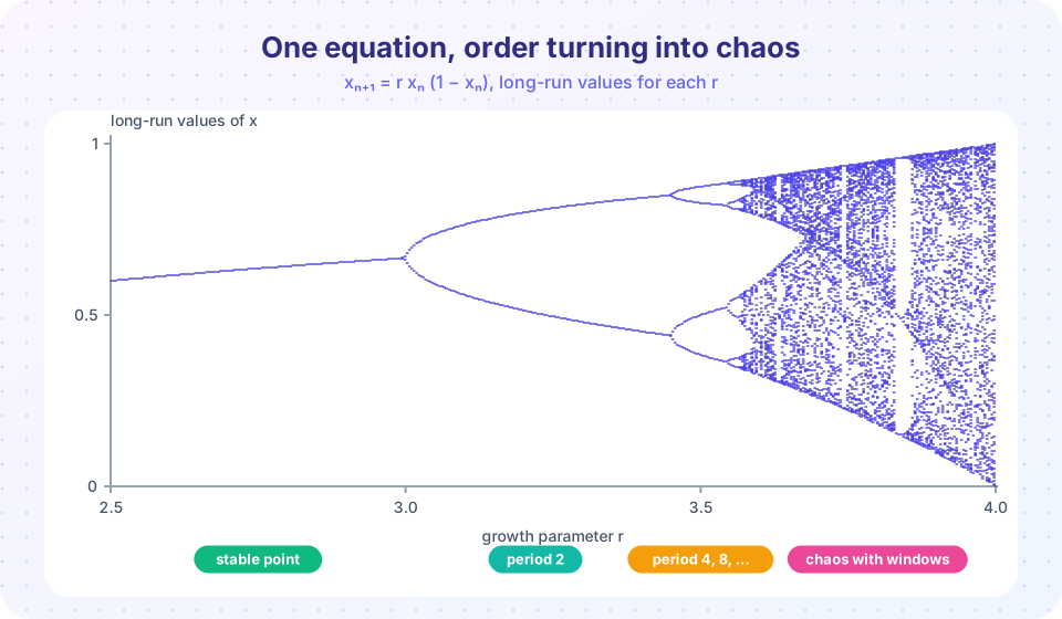
Reading it from left to right:
r < 1: extinction (x → 0).1 < r < 3: one stable population.r = 3: period doubling. The fixed point becomes unstable and a stable 2-cycle appears.r ≈ 3.449: the 2-cycle splits into a 4-cycle; then 8, 16, ... at closer and closer values ofr.r ≈ 3.5699: the cascade accumulates and chaos begins.- Inside the chaos there are windows of order. The most famous is a stable 3-cycle starting at
r = 1 + √8 ≈ 3.828.
In the 1970s Mitchell Feigenbaum discovered that the gaps between successive doublings shrink by a fixed factor, about 4.669, the same for a huge family of maps. That universal constant is now named for him.
Press Run (or Ctrl + Enter) to see the result here.
Program input · what you'd type while the program runs
Type the answers before you press Run, one per line. Each time the program reads a line (with input()), it gets the next line from this box.
Sensitive dependence
In the chaotic regime, two starting values that differ by a hair soon produce completely different histories. Meteorologist Edward Lorenz noticed this in 1961 while rounding numbers in a weather simulation, and later described its consequence as the "butterfly effect". The logistic map shows it in two lines of code.
The growth rate of tiny differences is measured by the Lyapunov exponent λ, the average of ln |f′(xₙ)| along an orbit. If λ > 0, nearby orbits separate exponentially: chaos. If λ < 0, they merge: stability.
Press Run (or Ctrl + Enter) to see the result here.
Program input · what you'd type while the program runs
Type the answers before you press Run, one per line. Each time the program reads a line (with input()), it gets the next line from this box.
A practical lesson follows: a chaotic model has a prediction horizon. If you can only measure the start to 6 digits, you lose all useful accuracy after a few dozen steps, however powerful your computer. Yet the model is still useful: it reveals the range, the typical behavior and the sensitivity itself.
Try it
Move the slider to change r, and watch the orbit. Try 2.8, 3.2, 3.5, 3.83 and 3.9.
Common misconceptions
"Chaos means randomness." The logistic map is completely deterministic: the same start always gives the same orbit. It only looks random because tiny differences are amplified.
"A chaotic model is useless." You lose long-term point prediction but keep the statistics, the bounds and the understanding of when the system is sensitive.
"Population really behaves like this." The logistic map is a toy model. It teaches what kinds of behavior simple rules allow. Real populations are shaped by many more effects, and few show clear chaos.
Check your understanding
Quick check · 5 questions
of 5 answered You scored / 5 · perfect!
-
1. What is the nonzero fixed point of x(n+1) = r x(n)(1 - x(n))?
Solving x = r x (1 - x) for x not equal to 0 gives 1 = r (1 - x), so x = 1 - 1/r. -
2. For which range of r is the positive fixed point of the logistic map stable?
The slope there is 2 - r, and |2 - r| < 1 exactly when 1 < r < 3. -
3. What happens at r = 3?
At r = 3 the slope at the fixed point is -1. Past it, a stable cycle of period 2 emerges. -
4. A positive Lyapunov exponent means:
Positive lambda means small differences grow exponentially, the hallmark of chaos. -
5. Which statement about chaos in the logistic map is correct?
The rule has no randomness, yet small errors grow so fast that long-term forecasts fail. For r up to 4, x stays in [0, 1].
Summary
- The logistic map
xₙ₊₁ = r xₙ(1 − xₙ)adds crowding to growth; its fixed points are0and1 − 1/r. - A fixed point is stable if
|f′(x*)| < 1; for the positive fixed point this means1 < r < 3. - Cobweb diagrams show iteration geometrically; the bifurcation diagram summarizes all long-run behaviors.
- Period doubling at
r = 3,≈ 3.449,≈ 3.544, ... leads to chaos nearr ≈ 3.57, with windows such as the 3-cycle atr ≈ 3.83. - Chaos is deterministic but has a prediction horizon, measured by a positive Lyapunov exponent.
Track your progress
Create a free account to tick off lessons and pick up where you left off on any device.
of Mathematical Modelling lessons completed