


















Lesson 23 of 46 · Continuous Models with ODEs
Logistic growth and harvesting
Model limits to growth with the logistic equation, find equilibria and stability with a phase line, and see how harvesting can sustain or collapse a population.
Exponential growth cannot last. A pond has a finite amount of food, a city has finite land, a virus runs out of people to infect. Real populations speed up when they are small, then slow down as they approach what their environment can support. The logistic equation, first proposed by the Belgian mathematician Pierre-François Verhulst in 1838, is the simplest model with this behaviour. Add a fishing quota to it and you get one of the most important lessons in resource management: a harvest that looks small can still destroy a population.
What you will learn
- How to write the logistic equation and read its parameters
randK. - How to find equilibria and decide whether they are stable using a phase line.
- How constant harvesting shifts the equilibria and can cause collapse.
- How to compare a closed-form solution with a numerical one.
Key terms
Carrying capacity (K): the population the environment can sustain, where growth stops.
Intrinsic growth rate (r): the per-capita growth rate when the population is tiny.
Stable equilibrium: an equilibrium that nearby solutions move toward.
Maximum sustainable yield: the largest harvest rate a population can support indefinitely.
From exponential to logistic
Start with the per-capita growth rate, the growth per individual. In the exponential model it is a constant r. Now let it shrink as the population N fills the habitat: r·(1 − N/K). It equals r when N is near zero and falls to zero when N = K. Multiply by N to get the total growth rate:
dN/dt = r · N · (1 − N/K)
This equation can be solved with separation of variables and partial fractions. With N(0) = N₀:
N(t) = K / (1 + ((K − N₀)/N₀) · e^(−r·t))
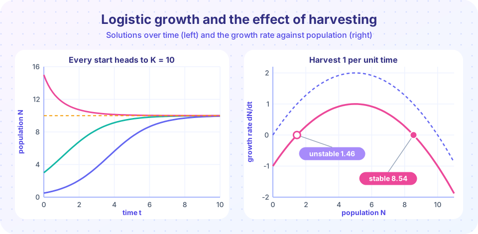
The graph is an S-curve. It starts nearly exponential, passes through its steepest point at N = K/2 (the inflection point), and levels off at K. If N₀ > K the curve falls toward K from above.
Equilibria and the phase line
You do not need the formula to understand the behaviour. Plot the growth rate g(N) = r·N·(1 − N/K) against N. It is a downward parabola that crosses zero at N = 0 and N = K. Those are the equilibria.
- Where
g(N) > 0the population increases (arrow pointing right on the number line). - Where
g(N) < 0it decreases (arrow pointing left).
Between 0 and K the arrows point right, toward K. Above K they point left, also toward K. So N = K is stable and N = 0 is unstable: a tiny population grows away from zero. The peak of the parabola is at N = K/2 and equals r·K/4. That number will matter in a moment.
Harvesting
Now remove individuals at a constant rate H (say fish caught per year):
dN/dt = r · N · (1 − N/K) − H
The curve is shifted down by H. The equilibria are the solutions of r·N·(1 − N/K) = H, a quadratic:
N = (K/2) · (1 ± √(1 − 4H/(r·K)))
Take r = 0.8 per year, K = 10 thousand fish, H = 1 thousand per year. The discriminant is 1 − 4/(8) = 0.5, so N = 5 · (1 ± 0.7071) = 1.46 or 8.54. The larger root is stable: the fishery settles at 8.54 thousand fish. The smaller root is unstable. If a bad winter pushes the population below 1.46 thousand, the harvest exceeds the births and the population collapses to zero.
The square root only exists when 4H ≤ r·K, that is when H ≤ r·K/4 = 2 thousand per year. That value is the maximum sustainable yield of a constant-quota fishery. Set the quota at 2.5 and there is no equilibrium at all: every starting population is driven to extinction, even a full one. Worse, at exactly H = 2 the single equilibrium (at K/2 = 5) is only half-stable: a small fluctuation downward leads to collapse.
Press Run (or Ctrl + Enter) to see the result here.
Program input · what you'd type while the program runs
Type the answers before you press Run, one per line. Each time the program reads a line (with input()), it gets the next line from this box.
Common misconceptions
"A population at the carrying capacity stops changing, so K is a limit that is never exceeded." K is an equilibrium, not a wall. A population above K (after a mild winter, say) decreases back toward it.
"If the quota is below the sustainable yield, the fishery is safe." Not if the population starts, or is pushed, below the unstable equilibrium. A constant quota ignores how many fish exist.
"Logistic growth is exactly how real populations behave." It is a first model. Delays, age structure and predators add oscillations that the logistic equation cannot show.
Proportional harvesting: a better policy
Instead of a fixed quota, fish with a fixed effort, so the catch is proportional to the population: dN/dt = r·N·(1 − N/K) − E·N. This is again a logistic equation, with growth rate r − E. The stable equilibrium is N* = K·(1 − E/r) and the yearly catch is E·N* = E·K·(1 − E/r). This parabola in E peaks at E = r/2, giving the same maximum yield r·K/4, but now a small population simply gets a small catch. The fishery cannot be driven to extinction as long as E < r. That is why many fisheries regulate effort or percentage of stock, not a fixed tonnage.
The next demo runs three constant quotas through the solver and shows where each ends up.
Press Run (or Ctrl + Enter) to see the result here.
Program input · what you'd type while the program runs
Type the answers before you press Run, one per line. Each time the program reads a line (with input()), it gets the next line from this box.
Phase-line explorer
Move the quota and watch the two equilibria approach each other and vanish.
Check your understanding
Quick check · 5 questions
of 5 answered You scored / 5 · perfect!
-
1. In dN/dt = r N (1 - N/K), what is the stable equilibrium?
Growth is positive below K and negative above K, so solutions move toward N = K. N = 0 is unstable. -
2. At what population is the logistic growth rate largest?
The growth rate rN(1 - N/K) is a parabola with its peak at N = K/2, where it equals rK/4. -
3. With r = 0.8 and K = 10, what is the maximum sustainable constant harvest?
H_max = rK/4 = 0.8 * 10 / 4 = 2. -
4. A fishery with a constant quota has an unstable equilibrium at 1.46 thousand fish. What happens if the stock falls to 1 thousand?
Below the unstable equilibrium the harvest exceeds growth, so the population keeps falling. -
5. Why is a harvest proportional to the stock safer than a fixed quota?
With catch E*N, a small population gets a small catch, so the population cannot be pushed to extinction while E is below r.
Summary
- The logistic equation
dN/dt = r·N·(1 − N/K)gives an S-curve with a stable equilibrium atK. - Equilibria are zeros of the growth rate; arrows on a phase line show stability.
- A constant harvest
Hcreates equilibria(K/2)(1 ± √(1 − 4H/(rK)))and vanishes aboverK/4. - Proportional (effort-based) harvesting is more robust than a fixed quota.
Track your progress
Create a free account to tick off lessons and pick up where you left off on any device.
of Mathematical Modelling lessons completed