


















Lesson 14 of 46 · Dimensional Analysis and Scaling
Scaling Laws and Allometry
Understand power laws y = a x^p, why they become straight lines on log-log plots, how to fit an exponent from data, and what Kleiber's 3/4 law says about animals.
Biologists noticed long ago that animals do not scale like cubes of jelly. Double an animal's mass and its need for energy does not double, and its heart does not beat twice as fast. Instead many properties follow power laws: simple relations of the form y = a x^p that hold over many orders of magnitude, from shrews to whales.
Power laws appear far beyond biology: city sizes, earthquake energies, the flow of rivers, the speed of computer programs. Learning to spot them, fit them and be careful with them is one of the most transferable skills in modelling.
What you will learn
- What a power law is and how its exponent
pis read from a log-log plot - How to fit an exponent with a straight-line fit in log coordinates
- What Kleiber's law says and why the geometry argument predicts a different exponent
- Why a good straight line on a log-log plot still needs caution
Key terms
Power law: a relation y = a x^p with constants a (the coefficient) and p (the exponent).
Log-log plot: a plot with logarithmic scales on both axes. A power law appears as a straight line with slope p.
Allometry: the study of how body features change with body size.
Isometric scaling: all parts scale in proportion to the geometry (area ∝ L², volume ∝ L³).
Scaling exponent: the number p that tells you how a quantity grows with size.
Power laws and straight lines
Take logarithms of y = a x^p:
log y = log a + p · log x
That is the equation of a straight line in the variables (log x, log y) with slope p and intercept log a. This is why scientists love log-log paper. A curve that is hard to judge by eye becomes a line, and the line's slope is the exponent.
Exponents tell stories:
Exponent p |
Meaning | Example |
|---|---|---|
p = 1 |
Proportional | Mass of a given material versus volume |
p = 2 |
Grows with area | Surface of a scaled shape versus length |
p = 3 |
Grows with volume | Mass of a scaled shape versus length |
0 < p < 1 |
Grows, but more slowly than size | Energy use of animals (about 3/4 of mass) |
p < 0 |
Decreases with size | Heart rate versus body mass (about −1/4) |
Kleiber's law
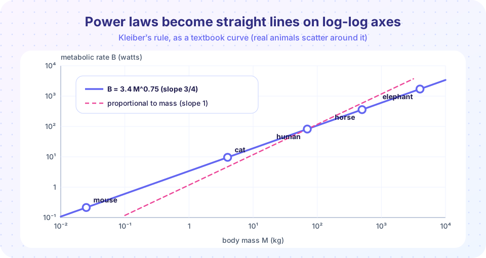
In 1932 the Swiss biologist Max Kleiber studied how the resting energy use of animals depends on body mass, using animals from rats up to cattle. He found that the metabolic rate B grows as the mass M to a power close to 3/4:
B ≈ B₀ M^(3/4)
A commonly quoted coefficient is about 3.4 W per kg^(3/4) for mammals, so B ≈ 3.4 M^(0.75) watts with M in kilograms. This is a typical textbook curve; real species scatter around it, and the details are debated.
Why is 3/4 surprising? A geometry-only argument says that heat is lost through the surface, so if animals were scaled copies, the heat they must make would scale like surface area: B ∝ M^(2/3) (this was the reasoning of Max Rubner in 1883). The observed exponent is a little bigger. In 1997 Geoffrey West, James Brown and Brian Enquist proposed that the branching networks that deliver blood and oxygen impose the extra factor, giving exactly 3/4. Other scientists argue that the true exponent varies between groups and conditions, so treat 3/4 as an approximation rather than a law of nature.
One consequence is easy to compute. The energy used per kilogram is B/M ∝ M^(−1/4). Small animals burn much more energy per gram than large ones, which is why a shrew must eat almost constantly.
Press Run (or Ctrl + Enter) to see the result here.
Program input · what you'd type while the program runs
Type the answers before you press Run, one per line. Each time the program reads a line (with input()), it gets the next line from this box.
Fitting an exponent from data
Given measurements (x_i, y_i), fit the exponent by fitting a straight line to (log x_i, log y_i): np.polyfit(np.log(x), np.log(y), 1) returns the slope p and intercept log a. This is quick and gives a good first estimate. Two cautions:
- Noise acts on the logarithm. The fit treats a 10% error at small
xthe same as a 10% error at largex. That is right when errors are proportional (multiplicative), which is common for biology, but wrong if errors are constant in size. - Quote an uncertainty. A single exponent without an error range is nearly useless. Bootstrapping gives one cheaply: refit many times on resampled data and look at the spread.
In the experiment below the data are synthetic, generated from a known exponent 0.75 with random scatter, so we can see how well the method recovers it.
Press Run (or Ctrl + Enter) to see the result here.
Program input · what you'd type while the program runs
Type the answers before you press Run, one per line. Each time the program reads a line (with input()), it gets the next line from this box.
A game: guess the exponent
Move the slider until the line goes through the middle of the points. The true exponent is hidden in the data. (Everything here is synthetic.)
Common misconceptions
"A straight line on log-log axes proves a power law." Many curves look straight over a short range, including lognormal and stretched-exponential shapes. Fit over several decades and compare with alternatives before claiming a power law.
"The exponent is a constant of nature." For biological scaling, estimates vary between species groups and methods. Report an interval, not a single sacred number.
"Big animals have lower metabolic rate." Their total rate is higher. Their rate per kilogram is lower, because p < 1.
Check your understanding
Quick check · 5 questions
of 5 answered You scored / 5 · perfect!
-
1. On a log-log plot, the power law y = a x^p appears as:
Taking logs gives log y = log a + p log x, a straight line of slope p. -
2. If B is proportional to M^(3/4), how does energy use per kilogram, B/M, change with mass?
B/M = M^(3/4 - 1) = M^(-1/4), so larger animals use less energy per kilogram. -
3. A simple surface-area argument for heat loss predicts which metabolic exponent?
Surface scales as length squared and mass as length cubed, so surface goes as mass to the power 2/3. -
4. Mass is multiplied by 16. By what factor does B = 3.4 M^(3/4) grow?
16^(3/4) = (16^(1/4))^3 = 2^3 = 8. -
5. You fit a slope on a log-log plot and get 0.74 from 10 points. What should you do next?
A single exponent without an error range or model check is not trustworthy.
Summary
- A power law
y = a x^pis a straight line of slopepon log-log axes. - Fit exponents with
np.polyfit(np.log(x), np.log(y), 1)and always add an uncertainty, for example from a bootstrap. - Kleiber's rule
B ∝ M^(3/4)is a textbook approximation; geometry alone suggests2/3, and the debate is still open. - Energy per kilogram falls with size as
M^(−1/4). - Straight lines on log-log plots can mislead; check range and alternatives.
Next: Chapter 3 Review
Track your progress
Create a free account to tick off lessons and pick up where you left off on any device.
of Mathematical Modelling lessons completed