


















Lesson 19 of 46 · Discrete Dynamical Models
Matrix Models: Leslie and Markov
Model age-structured populations with Leslie matrices and random state changes with Markov chains: growth rates, stable distributions and what-if experiments.
So far each model tracked a single number. But many systems have several interacting quantities: juveniles and adults, sunny and rainy days, healthy and infected people. To handle several at once, the state becomes a list of numbers (a vector) and the update rule becomes matrix multiplication: xₙ₊₁ = A xₙ.
This one idea covers an enormous range of models, and linear algebra gives you powerful answers about them for free.
What you will learn
- How to build a Leslie matrix for an age-structured population
- How the dominant eigenvalue gives the long-run growth rate and the eigenvector the stable age distribution
- What a Markov chain is and how to find its steady state
- How to run what-if experiments with matrix models
Key terms
State vector xₙ: a list of quantities (for example, number of animals in each age class).
Leslie matrix L: a matrix of birth rates (first row) and survival rates (just below the diagonal) that advances age classes by one time step.
Eigenvalue and eigenvector: a number λ and vector v with A v = λ v; the matrix only stretches v by λ.
Markov chain: a model where the next state depends only on the current state, with fixed transition probabilities.
Stable distribution: the long-run mix of states that no longer changes shape.
The Leslie matrix
In 1945 the biologist Patrick Leslie proposed a model for populations divided into age classes. Take three classes: juveniles x₁, young adults x₂, adults x₃, counted once a year.
- Fecundity
fⱼ: average number of offspring (who start as juveniles next year) per individual in classj. - Survival
sⱼ: probability that an individual in classjsurvives to classj + 1.
Next year's classes are
x₁' = f₂ x₂ + f₃ x₃ (births), x₂' = s₁ x₁, x₃' = s₂ x₂
In matrix form xₙ₊₁ = L xₙ:
L = [[0, f₂, f₃], [s₁, 0, 0], [0, s₂, 0]]
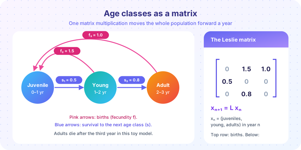
With the toy values f₂ = 1.5, f₃ = 1.0, s₁ = 0.5, s₂ = 0.8, the matrix is the one on the right of the picture (these are illustrative numbers, not data for a real species).
What happens in the long run?
Linear algebra gives a clear answer. Repeated multiplication makes the state line up with the dominant eigenvector of L, and from then on each year multiplies the whole population by the dominant eigenvalue λ:
λ > 1: the population grows by about(λ − 1)per yearλ = 1: it holds steadyλ < 1: it declines
The eigenvector, scaled to sum to one, is the stable age distribution: the share of each class in the long run, whatever the starting mix.
Press Run (or Ctrl + Enter) to see the result here.
Program input · what you'd type while the program runs
Type the answers before you press Run, one per line. Each time the program reads a line (with input()), it gets the next line from this box.
After a few oscillating years the total grows by a steady ratio equal to λ, and the age shares reach the dotted lines.
A what-if experiment
Conservation biologists use exactly this tool to ask which stage matters most. Suppose juvenile survival s₁ drops (pollution, predators). At what value does the population stop growing? The net reproductive rate R₀ = s₁ (f₂ + f₃ s₂), the expected number of offspring per newborn over its life, tells you: λ = 1 precisely when R₀ = 1.
Press Run (or Ctrl + Enter) to see the result here.
Program input · what you'd type while the program runs
Type the answers before you press Run, one per line. Each time the program reads a line (with input()), it gets the next line from this box.
Markov chains: when change is random
A Markov chain (named for Andrey Markov, who studied them around 1906) moves between states with fixed probabilities. Example: each day is sunny or rainy; after a sunny day it is sunny again with probability 0.8, after a rainy day it is sunny with probability 0.4. Collect the probabilities in a transition matrix, one row per current state:
P = [[0.8, 0.2], [0.4, 0.6]]
If πₙ is the row vector of probabilities of being sunny or rainy on day n, then πₙ₊₁ = πₙ P. The steady state π* satisfies π* P = π*: the left eigenvector for eigenvalue 1. Solving by hand gives π* = (2/3, 1/3): in the long run two days in three are sunny, whatever today's weather. The probabilities are a toy example, not a forecast.
Press Run (or Ctrl + Enter) to see the result here.
Program input · what you'd type while the program runs
Type the answers before you press Run, one per line. Each time the program reads a line (with input()), it gets the next line from this box.
Notice the difference in spirit. The Leslie model is deterministic and tracks amounts; the Markov chain tracks probabilities, and a single run is random. Chapter 7 returns to simulating such chance processes.
Common misconceptions
"Eigenvalues are only abstract mathematics." Here the dominant eigenvalue is the yearly growth factor of a population: a number a conservation manager can act on.
"The age shares settle immediately." There is usually a transient with oscillations before the stable distribution appears. Early projections can mislead.
"A matrix model predicts the real population." It predicts what happens if rates stay constant forever. Real rates change with weather, density and disease.
Check your understanding
Quick check · 5 questions
of 5 answered You scored / 5 · perfect!
-
1. In a Leslie matrix, the first row holds:
The first row produces the new juveniles, from the fecundities of each class. Survival rates sit just below the diagonal. -
2. If the dominant eigenvalue of a Leslie matrix is 0.93, the population:
Each year the long-run population is multiplied by 0.93, a loss of 7%. -
3. What does the dominant eigenvector (scaled to sum 1) represent?
It gives the long-run share of each age class. -
4. A Markov chain has transition matrix rows (0.9, 0.1) and (0.5, 0.5). What is the steady probability of state 1?
Steady state: pi1 = pi10.9 + pi20.5 with pi1 + pi2 = 1, so 0.1 pi1 = 0.5 (1 - pi1), 0.6 pi1 = 0.5, pi1 = 5/6. -
5. Which statement about Markov chains is true?
That is the Markov property: the future depends on the past only through the present.
Summary
- Vectors and matrices let discrete models track several quantities:
xₙ₊₁ = A xₙ. - A Leslie matrix has fecundities in the first row and survival rates below the diagonal.
- The dominant eigenvalue is the long-run growth factor; its eigenvector is the stable age distribution;
R₀ = 1marks the threshold. - A Markov chain moves between states with fixed probabilities; its steady state is the left eigenvector for eigenvalue 1.
Next: Chapter 4 Review
Track your progress
Create a free account to tick off lessons and pick up where you left off on any device.
of Mathematical Modelling lessons completed