


















Lesson 45 of 46 · Projects and Practice
Cheat sheet: chapters 5 to 8 on one page
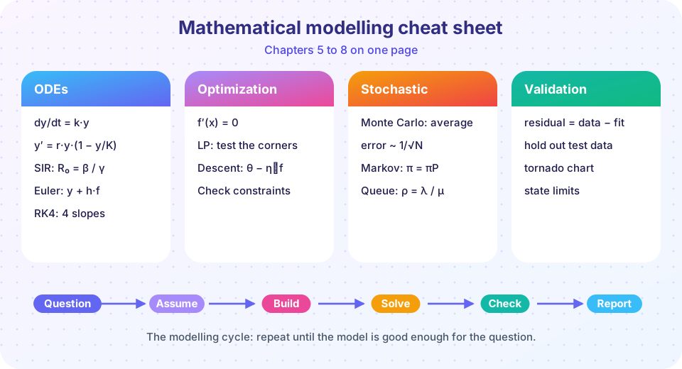
A one-page recap of the key formulas and checks for ODE models, optimization, stochastic simulation and validation, with a poster and runnable calculators.
This page is the one you will come back to. It puts the key formulas and habits of the second half of the course on a poster and in a table, and gives you a handful of small calculators so you can check numbers quickly. Print it, or keep it open while you work on a model.
What you will learn
- Where to find each key formula in a second.
- Which check to run before you trust an answer.
- How to use small calculators for common questions.
Key terms
Cycle: question, assume, build, solve, check, report; repeat until the model is good enough.
Sanity check: a quick test on units, size and limiting cases.
Formula card: a short list of equations you can use without rederiving them.
Formulas
| Topic | Formula | Notes |
|---|---|---|
| Exponential | y = y₀·e^(k·t) |
half-life is ln 2 divided by the size of k |
| Newton cooling | T = T_env + (T₀ − T_env)·e^(−k·t) |
gap decays exponentially |
| Logistic | N(t) = K / (1 + ((K − N₀)/N₀)·e^(−r·t)) |
fastest growth at K/2 |
| Harvesting | H_max = r·K/4; N* = K(1 − E/r) |
constant versus proportional |
| SIR | R₀ = β/γ; peak at S = 1/R₀ |
threshold 1 − 1/R₀ immune |
| Lotka-Volterra | equilibrium (c/d, a/b) |
closed cycles |
| Euler | y + h·f(t, y) |
error ∝ h |
| RK4 | y + (h/6)(k₁ + 2k₂ + 2k₃ + k₄) |
error ∝ h⁴ |
| Calculus optimum | f′(x) = 0, check f″ and ends |
can: h = 2r |
| LP | optimum at a corner | shadow price = value of a binding unit |
| Gradient descent | θ ← θ − η·∇f |
stable if η < 2/λ_max |
| Monte Carlo | error ≈ σ/√N |
100× samples, 10× precision |
| Random walk | spread √n |
fair ruin: k/N |
| Markov chain | π·P = π, rows sum to 1 |
spell length 1/(1 − a) |
| M/M/1 | ρ = λ/μ, W_q = ρ/(μ − λ), L = λ·W |
explodes as ρ → 1 |
| Least squares | m = S_xy/S_xx, c = ȳ − m·x̄ |
R² = 1 − SSE/SST |
| Elasticity | (Δout/out)/(Δin/in) |
above 1 amplifies |
The gradient-descent stability rule: for a quadratic loss with largest curvature λ_max (largest eigenvalue of the Hessian), the learning rate must be below 2/λ_max. For x² + 5y² the Hessian eigenvalues are 2 and 10, so η < 0.2.
Three checks before you trust a result
- Units and limits. Do the units balance? Does the model give the right answer when a parameter is zero or very large?
- A second method. Solve it a second way: a formula and a simulation, or two step sizes.
- A range. Change the main inputs by 10 percent and report the resulting range.
Calculators
Press Run (or Ctrl + Enter) to see the result here.
Program input · what you'd type while the program runs
Type the answers before you press Run, one per line. Each time the program reads a line (with input()), it gets the next line from this box.
The second tool draws the phase of the modelling cycle that you most often skip: a sensitivity bar chart from any numbers you provide. Replace the dictionary with your own model's inputs and outputs.
Press Run (or Ctrl + Enter) to see the result here.
Program input · what you'd type while the program runs
Type the answers before you press Run, one per line. Each time the program reads a line (with input()), it gets the next line from this box.
Look at price: it is already at its best value, so moving it either way loses exactly the same profit, and the two printed profits are equal. A tornado chart shows the loss from moving an input, so the bar for an input at its optimum extends only to one side. That is the flat top of the profit curve from Chapter 6 in another guise.
Check your understanding
Quick check · 5 questions
of 5 answered You scored / 5 · perfect!
-
1. Which formula gives the largest sustainable constant harvest of a logistic population?
The growth rate peaks at N = K/2 where it equals rK/4. -
2. For a quadratic loss with largest Hessian eigenvalue 10, the learning rate must be below:
The condition is eta < 2 / lambda_max = 2/10. -
3. A simulation's error is 0.05 with 10,000 runs. About how many runs give an error of 0.005?
10 times less error needs 100 times more runs. -
4. Which check helps catch a wrong formula?
Independent methods that agree build confidence; disagreement reveals mistakes. -
5. In M/M/1 with rho = 0.5 and mu = 1, the wait in line Wq is:
Wq = rho / (mu - lambda) = 0.5 / 0.5 = 1.
Summary
- Keep the formula table and the three checks next to every model.
- Use calculators to test numbers fast; confirm with a second method.
- A tornado chart ranks which inputs deserve attention.
- The cycle never ends: question, assume, build, solve, check, report, repeat.
Track your progress
Create a free account to tick off lessons and pick up where you left off on any device.
of Mathematical Modelling lessons completed