


















Lesson 20 of 46 · Discrete Dynamical Models
Chapter 4 Review: Discrete Dynamical Models
Review chapter 4: difference equations, fixed points and stability, the logistic map, and matrix models. A one-page cobweb picture, a Ricker model exercise and a quiz.
This chapter showed that a state, an update rule and a starting value are enough to model anything that changes in steps. You solved linear rules exactly, found where nonlinear rules settle and why they sometimes do not, and handled several quantities at once with matrices.
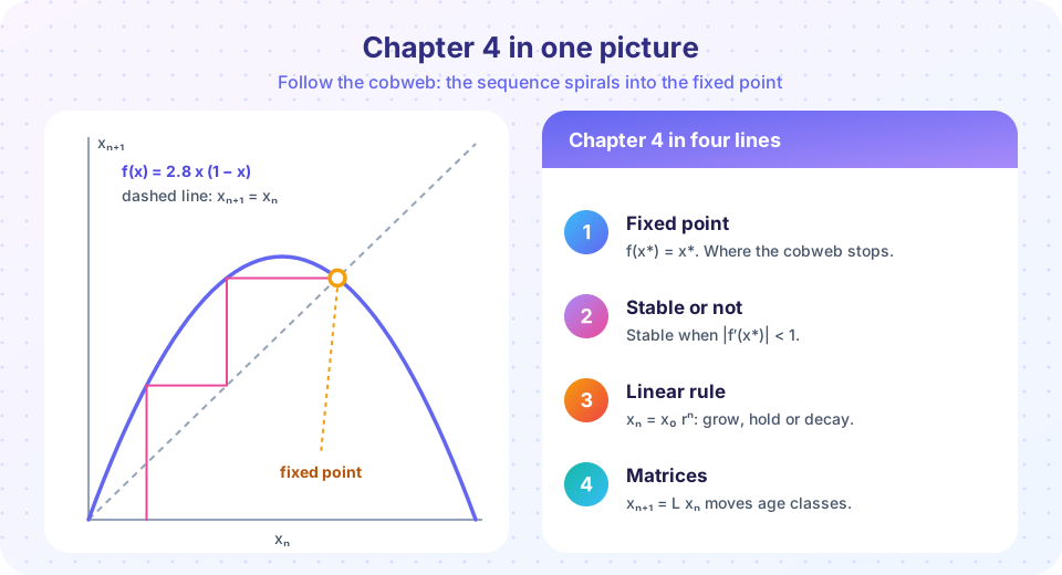
The chapter in a table
| Lesson | Key idea | Formula |
|---|---|---|
| Overview | State, rule and initial condition generate the future | xₙ₊₁ = f(xₙ) |
| Difference Equations and Their Solutions | Linear rules are solvable; stable if |r| < 1 |
xₙ = x* + rⁿ(x₀ − x*), x* = b/(1 − r) |
| The Logistic Map and Chaos | Stability from the slope; period doubling; sensitivity | x* = 1 − 1/r, stable for 1 < r < 3 |
| Matrix Models: Leslie and Markov | Eigenvalue = growth rate, eigenvector = stable shares | xₙ₊₁ = L xₙ, π P = π |
The three-step stability recipe
- Find fixed points: solve
f(x*) = x*. - Compute the slope
f′(x*). - Decide: stable if
|f′(x*)| < 1, unstable if|f′(x*)| > 1. Iff′ < 0the approach oscillates; iff′ > 0it is monotone.
Try it
Automate the recipe. The function below finds fixed points numerically for any one-variable rule and classifies them, so you can test models you have never seen.
Press Run (or Ctrl + Enter) to see the result here.
Program input · what you'd type while the program runs
Type the answers before you press Run, one per line. Each time the program reads a line (with input()), it gets the next line from this box.
The Ricker model, devised by the fisheries scientist William Ricker in 1954 for fish stocks, is another crowding rule. Its fixed point x* = 1 has slope f′(1) = 1 − r, so it is stable for 0 < r < 2. Let us confirm with a bifurcation diagram: before r = 2 one branch, after it period doubling again.
Press Run (or Ctrl + Enter) to see the result here.
Program input · what you'd type while the program runs
Type the answers before you press Run, one per line. Each time the program reads a line (with input()), it gets the next line from this box.
That the logistic and Ricker maps look so alike, despite different formulas, hints at something deep: the structure (a hump-shaped rule with one maximum) matters more than the formula. Feigenbaum's constant is the same for both.
Check your understanding
Quick check · 10 questions
of 10 answered You scored / 10 · perfect!
-
1. A fixed point x* of x(n+1) = f(x(n)) satisfies:
If the state equals x*, the next state is f(x*) = x*, so nothing changes. -
2. x(n+1) = 0.9 x(n) + 2. The equilibrium and its stability are:
x* = 2 / (1 - 0.9) = 20, and |0.9| < 1 so it is stable. -
3. The slope at a fixed point is f'(x*) = -0.6. The sequence approaches x*:
|slope| < 1 means stable. A negative slope means the deviation flips sign each step. -
4. For the logistic map, the nonzero fixed point loses stability at r = :
The slope there is 2 - r, which equals -1 at r = 3, the first period doubling. -
5. For a Leslie matrix with dominant eigenvalue 1.06, the population grows by about:
A factor 1.06 per step is a 6% increase. -
6. A loan balance follows B(n+1) = 1.004 B(n) - 150. Starting balance 20,000. P/i = 150/0.004 = 37,500. What happens?
The start is below the unstable equilibrium 37,500, so deviations grow downward and the balance falls to zero. -
7. Which of these is a sign of chaos in a deterministic model?
A positive exponent means nearby orbits separate exponentially: sensitive dependence. -
8. The Fibonacci sequence's ratio of consecutive terms tends to:
It tends to the golden ratio, the positive root of x^2 = x + 1. -
9. Net reproductive rate R0 for a Leslie model equals 0.9. What does this imply?
R0 < 1 means each newborn is replaced by fewer than one offspring on average, so lambda < 1. -
10. In a Markov chain, the steady-state vector satisfies:
Multiplying the distribution by the transition matrix leaves it unchanged.
Summary
- Fixed points solve
f(x*) = x*; they are stable when|f′(x*)| < 1. - Linear rules
xₙ₊₁ = r xₙ + bhave closed forms; the loan and Fibonacci are examples. - The logistic and Ricker maps show period doubling and chaos; chaos is deterministic with a prediction horizon.
- Leslie matrices give growth rate (eigenvalue) and stable age shares (eigenvector); Markov chains have steady states with
π P = π. - Next chapter: the same ideas with continuous time, using differential equations.
Track your progress
Create a free account to tick off lessons and pick up where you left off on any device.
of Mathematical Modelling lessons completed