


















Lesson 41 of 46 · Projects and Practice
Project: fit and forecast an outbreak
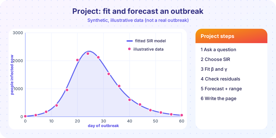
A complete modelling project: fit an SIR model to the early days of a synthetic outbreak, forecast the rest, test the forecast and see why early data cannot pin down every parameter.
This project uses almost everything in the course. You will receive daily counts from the first weeks of an outbreak and have to answer a decision-maker's question: when will the number of people sick at once peak, and how large will it be? You will build and fit an SIR model, test the forecast against the days you held back, and discover the main reason why early forecasts are hard.
What you will learn
- How to carry a modelling project from question to report.
- How to fit an ODE model to data with
least_squares. - How to test a forecast with data held back.
- Why different parameter sets can fit the early data equally well yet forecast very differently.
Key terms
Synthetic data: data generated by a model with known parameters, used to test methods because we know the truth.
Identifiability: whether the data contain enough information to determine each parameter separately.
Forecast horizon: how far ahead a prediction reaches.
Hold-out data: observations kept out of the fit and used to test it.
Step 1: the question and the data
The town has 10,000 people. A health officer wants to know when the number of currently infected people peaks and how high it goes, so that beds can be prepared. We have daily counts of currently infected people for days 0 to 14, two weeks into the outbreak. (The data below are synthetic: we generate them from an SIR model with β = 0.45 and γ = 0.18 and add 10 percent random noise. Using synthetic data lets us check our answer against the truth, which real outbreaks never allow.)
The model is the SIR model from Chapter 5 with counts instead of fractions:
dS/dt = −β·S·I/N, dI/dt = β·S·I/N − γ·I, dR/dt = γ·I
with N = 10,000 and I(0) = 20. The unknowns are β and γ.
Step 2: fit
We choose β and γ to minimize the squared difference between log(observed) and log(model). Logs are used because the noise is proportional (10 percent of the size), so an error of 100 when I is 2,000 matters no more than an error of 1 when I is 20.
Press Run (or Ctrl + Enter) to see the result here.
Program input · what you'd type while the program runs
Type the answers before you press Run, one per line. Each time the program reads a line (with input()), it gets the next line from this box.
Step 3: check the residuals and the hold-out data
A fit that looks good on the days it was trained on is not yet a forecast you can trust. Compare the forecast with the held-out days 15 to 60. Look at the residuals of the fitted period too: they should look like random noise with a standard deviation near 0.10 on the log scale, because that is how we generated the data.
Step 4: why early data are ambiguous
In the early phase almost everyone is susceptible, so S ≈ N and the equation for I becomes approximately dI/dt ≈ (β − γ)·I: exponential growth at rate β − γ. The early data therefore pin down the growth rate β − γ accurately, but they say little about β and γ separately. Yet the shape of the peak depends on R₀ = β/γ. A pair with a smaller γ and a smaller β can grow at the same early rate and then reach a very different peak.
The next experiment shows this directly. We fix γ at three plausible values (0.10, 0.18 and 0.30), fit β to the same early data each time, and compare the fits and their forecasts.
Press Run (or Ctrl + Enter) to see the result here.
Program input · what you'd type while the program runs
Type the answers before you press Run, one per line. Each time the program reads a line (with input()), it gets the next line from this box.
Common misconceptions
"A good fit means a good forecast." The three fits above are nearly equally good on the data used, yet their predictions diverge. Fit quality on training data says nothing about the parameters that the data cannot constrain.
"The best-fit parameters are the true ones." With noisy, short data, the best-fit parameters can be far from the truth in the directions the data do not constrain.
"More complex models will fix it." Extra parameters make the identifiability problem worse. The remedy is more data, outside information (for example the infectious period of the disease, which fixes γ) and honest ranges.
Step 5: what would you report?
Answer the health officer in a few lines:
- Question: peak time and size of currently infected people.
- Result: the early data fix the growth rate, but the peak size depends on
R₀, which they do not pin down. Give a range that covers the plausibleγvalues, not one curve. - Better data: the length of time people stay infectious, measured in a small clinical study, would shrink the range the most (this is what the sensitivity analysis of Chapter 8 predicts).
- Limits: equal mixing, no behaviour change, no interventions.
A good report, in the five-part format from the previous lesson, fits on one page.
Check your understanding
Quick check · 5 questions
of 5 answered You scored / 5 · perfect!
-
1. In the early phase of an SIR outbreak, which combination do the data constrain best?
While almost everyone is susceptible, I grows like exp((beta - gamma) t). -
2. Why is the fit done on the logarithm of the counts?
With multiplicative noise, residuals on the log scale have roughly constant spread. -
3. What does synthetic data allow you to do?
Because we generated the data, we know the true parameters and can test the method. -
4. Three parameter sets fit the early data equally well but forecast very different peaks. What should you report?
When parameters are not identifiable, honest reporting gives the range and the data needed to reduce it. -
5. Which outside information would best fix gamma in an epidemic model?
gamma is the reciprocal of the mean infectious period.
Summary
- A project follows the cycle: question, model, fit, check, forecast, report.
- Early outbreak data constrain the growth rate
β − γ, notβandγseparately. - Different parameter sets can fit equally well and forecast very differently.
- Report a range, name the data that would narrow it, and state the limits.
Track your progress
Create a free account to tick off lessons and pick up where you left off on any device.
of Mathematical Modelling lessons completed