


















Lesson 34 of 46 · Stochastic Models and Simulation
Queue simulation: waiting lines and the load ρ
Simulate single-server queues from arrival and service times, compare with the M/M/1 formulas, and see why waits explode as the load approaches one.
Supermarket checkouts, call centres, hospital emergency rooms, web servers: wherever customers arrive at random and servers take random time, queues form. Even when the server is idle some of the time, randomness makes people wait. The mathematics of queues was started by the Danish engineer Agner Krarup Erlang, who studied telephone exchanges in the early 1900s. In this lesson you will simulate a queue from first principles, compare it with the classic formulas, and discover the most important rule in the subject: delays blow up as the server gets close to full.
What you will learn
- How to simulate a single-server queue with a simple recursion.
- The M/M/1 formulas for load, average queue wait and system time.
- Why waiting time grows so fast as the load
ρapproaches 1. - How one fast server compares with two slower servers.
Key terms
Arrival rate (λ): average number of customers arriving per unit time.
Service rate (μ): average number of customers one server can finish per unit time.
Utilization or load (ρ = λ/μ): the fraction of time the server is busy.
M/M/1 queue: one server, random (Poisson) arrivals and exponentially distributed service times; the first M's stand for "memoryless".
Simulating a queue
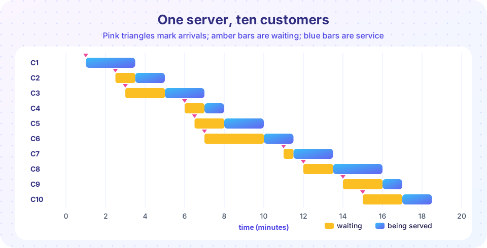
You do not need an advanced library. Keep a record of when the server becomes free. For customer i with arrival time aᵢ and service time sᵢ:
start_i = max(a_i, previous finish)wait_i = start_i − a_ifinish_i = start_i + s_i
The timeline above has ten customers with arrival times 1, 2.5, 3, 6, 6.5, 7, 11, 12, 14, 15 minutes and service times 2.5, 1.5, 2, 1, 2, 1.5, 2, 2.5, 1, 1.5 minutes. Customer 2 arrives at 2.5 but the server is busy until 3.5, so they wait one minute. The ten waits are 0, 1, 2, 1, 1.5, 3, 0.5, 1.5, 2, 2: an average of 1.45 minutes. In this run the server is busy without a break from minute 1 to minute 18.5, so the line never empties. Arrivals bunch up (three customers in the minutes 6 to 7) and the bunch has to be worked off.
Press Run (or Ctrl + Enter) to see the result here.
Program input · what you'd type while the program runs
Type the answers before you press Run, one per line. Each time the program reads a line (with input()), it gets the next line from this box.
The M/M/1 formulas
Now let arrivals be random (the gaps between customers follow an exponential distribution with mean 1/λ) and service times also exponential with mean 1/μ. The system is stable only if ρ = λ/μ < 1. Then, on average:
- customers waiting in line:
L_q = ρ² / (1 − ρ) - time waiting in line:
W_q = ρ / (μ − λ) - time in the system (wait plus service):
W = 1 / (μ − λ) - customers in the system:
L = ρ / (1 − ρ)
These obey Little's law, L = λ·W, one of the most useful identities in operations research.
Take λ = 0.8 customers per minute and μ = 1 per minute, so ρ = 0.8. Then W_q = 0.8/0.2 = 4 minutes and W = 5 minutes. At ρ = 0.9, W_q = 9 minutes; at ρ = 0.95, 19 minutes. The service time never changed, but waiting time exploded. The last few percent of utilization are extremely expensive, which is why well-run services keep a buffer of spare capacity, and why a motorway jams suddenly when traffic increases only a little.
To simulate, use the recursion for waits: if W_i is the wait of customer i, then W_i = max(0, W_{i−1} + S_{i−1} − A_i), where A_i is the gap between arrivals i − 1 and i.
Press Run (or Ctrl + Enter) to see the result here.
Program input · what you'd type while the program runs
Type the answers before you press Run, one per line. Each time the program reads a line (with input()), it gets the next line from this box.
Common misconceptions
"If the server is busy 80 percent of the time, customers wait 80 percent of a service time." Waiting depends on randomness, not only on load. At 80 percent load the average wait is four service times in the M/M/1 model.
"Adding a little capacity does little." Near full load a small increase in capacity cuts waits sharply, for the same reason that a small increase in load raises them sharply.
"If average arrivals are below average capacity, there is no queue." Averages hide bunching. Random gaps and random service times create queues even when ρ is well below 1.
One fast server or two slow ones?
A shop receives λ = 1.6 customers per minute. Option A: one server with μ = 2 per minute. Option B: two servers, each with μ = 1 per minute. Both have the same total capacity of 2 and the same load ρ = 0.8. Which is better? Theory says it depends on what you measure. With two servers a customer is more likely to find someone free, so the wait in the line is shorter. But the one fast server completes each job twice as quickly, so the total time in the system is shorter. Simulation lets you see both.
Press Run (or Ctrl + Enter) to see the result here.
Program input · what you'd type while the program runs
Type the answers before you press Run, one per line. Each time the program reads a line (with input()), it gets the next line from this box.
Check your understanding
Quick check · 5 questions
of 5 answered You scored / 5 · perfect!
-
1. Customers arrive at 0.8 per minute and one server completes 1 per minute. What is the load rho?
rho = lambda / mu = 0.8 / 1 = 0.8. -
2. For an M/M/1 queue with rho = 0.9 and mu = 1 per minute, what is the average wait in line?
Wq = rho / (mu - lambda) = 0.9 / 0.1 = 9 minutes. -
3. What happens if rho is above 1?
Arrivals exceed capacity on average, so the line keeps growing. -
4. In the 10-customer example, customer 2 arrives at 2.5 and the server is free at 3.5. How long do they wait?
Wait = start - arrival = 3.5 - 2.5 = 1 minute. -
5. Little's law says that, in steady state:
The average number in the system equals the arrival rate times the average time in the system.
Summary
- Simulate a queue with
start = max(arrival, server free),wait = start − arrival. - M/M/1:
ρ = λ/μ,W_q = ρ/(μ − λ),W = 1/(μ − λ),L = λW. - Waits grow without bound as
ρ → 1; keep spare capacity. - Pooling servers lowers queue wait but a single fast server lowers total time: pick the metric first.
Next: Chapter 7 review
Track your progress
Create a free account to tick off lessons and pick up where you left off on any device.
of Mathematical Modelling lessons completed