


















Lesson 21 of 46 · Continuous Models with ODEs
Chapter 5 overview: continuous models with ODEs
See the big picture of modelling with ordinary differential equations: growth, logistic limits, epidemics and numerical solvers, and how the lessons fit together.
So far you have built models from tables, formulas and step-by-step rules. In this chapter you meet the most powerful tool for things that change smoothly: the ordinary differential equation, or ODE. Instead of describing where a quantity is, an ODE describes how fast it is changing right now. From that one sentence you can recover the whole story of a cooling cup of coffee, a growing colony of bacteria, or an epidemic sweeping through a town.
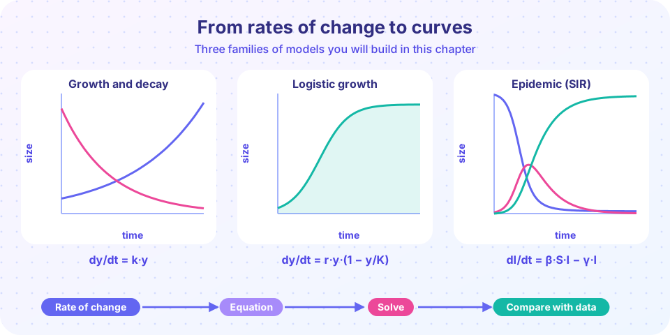
What you will learn
- Why a rate of change is often easier to model than the quantity itself.
- How to read an ODE as a recipe: "the speed of change depends on the current state".
- The four model families you will build: exponential, logistic, coupled systems and numerical solutions.
- How the lessons of this chapter connect to the optimization and stochastic models that follow.
Key terms
Ordinary differential equation (ODE): an equation that relates a function of one variable (usually time) to its own derivatives.
Initial value problem: an ODE together with the starting value of the quantity, which picks out one solution.
Equilibrium: a value of the state at which the rate of change is zero, so nothing moves.
Numerical solution: a table of approximate values built step by step by a computer.
Why rates are the natural starting point
Ask yourself how a bathtub fills. You rarely know the water depth as a formula in time, but you know what is happening this second: water flows in at a certain rate and drains out at a certain rate. The change in volume is "in minus out". Writing that sentence in symbols gives an ODE, dV/dt = in − out.
This is the central modelling habit of the chapter. Do not try to guess the curve. Describe the forces that push it, and let mathematics produce the curve. The same habit works for money in a savings account, drug in the bloodstream, people in a city and rabbits in a field.
The four ideas of the chapter
Rates first
Growth and decay
Limits to growth
Systems
Always check
What each lesson covers
- Growth, decay and Euler's method: the model
dy/dt = k·y, Newton's law of cooling, half-life, and your first numerical solver. - Logistic growth and harvesting: limits to growth, equilibria, stability, and what fishing quotas do to a population.
- SIR epidemics and predator-prey systems: two or three coupled equations, the basic reproduction number and the phase plane, solved with Runge-Kutta.
- Chapter review: a one-page summary and a long quiz.
Try it
The first demo shows the single idea behind every lesson here: given only a rule for the slope, a computer can draw the curve. Change the numbers and watch the shape change.
Press Run (or Ctrl + Enter) to see the result here.
Program input · what you'd type while the program runs
Type the answers before you press Run, one per line. Each time the program reads a line (with input()), it gets the next line from this box.
Check your understanding
Quick check · 4 questions
of 4 answered You scored / 4 · perfect!
-
1. What does an ordinary differential equation describe?
An ODE relates a derivative, the rate of change, to the current state and time. -
2. A bathtub gains 12 litres per minute from the tap and loses 8 litres per minute down the drain. What is dV/dt?
dV/dt equals inflow minus outflow: 12 - 8 = 4 litres per minute. -
3. What is an equilibrium of an ODE?
At an equilibrium dy/dt = 0, so the solution stays where it is. -
4. Why do we often solve ODEs numerically?
Most realistic models have no closed-form solution, but a computer can follow the slope step by step.
Summary
- An ODE says how fast something changes given its current state.
- Model the forces that push the quantity; let the mathematics build the curve.
- This chapter covers exponential, logistic, coupled systems and numerical solvers.
- Always compare the solution with data or with a simpler check.
Track your progress
Create a free account to tick off lessons and pick up where you left off on any device.
of Mathematical Modelling lessons completed