


















Lesson 28 of 46 · Optimization Models
Linear programming models
Formulate and solve linear programs: write constraints and an objective, find the best corner point of the feasible region, and read slack and shadow prices.
Calculus works when you have one smooth curve. But businesses, hospitals and farms face many limits at once: hours, money, materials, space. If every limit and the goal are linear (straight-line relationships), you have a linear program, and one remarkable fact solves it: the best answer is always at a corner of the feasible region. Linear programming was developed in the 1940s (George Dantzig's simplex method dates from 1947) and still schedules airlines, mixes animal feed and routes oil, today with millions of variables.
What you will learn
- How to turn a word problem into a linear program.
- How to find the optimum graphically and by checking corner points.
- What slack and binding constraints mean.
- What a shadow price tells a manager, and when it stops being valid.
Key terms
Linear program (LP): maximize or minimize a linear objective subject to linear constraints.
Corner point (vertex): a feasible point where two or more constraint lines meet.
Binding constraint: a constraint that holds with equality at the optimum, using up its resource.
Shadow price: the gain in the objective from one extra unit of a binding resource.
Formulating the problem
A small workshop makes two products. Let x be the number of batches of tables and y the number of batches of chairs per day.
- A table batch earns 3 (hundred dollars); a chair batch earns 2.
- Wood: each batch of either product uses 1 sheet and 4 sheets are available.
- Carpentry: a table batch takes 1 hour and a chair batch takes 3 hours; 7 hours are available.
- The finishing machine can handle at most 3 table batches.
Model. Maximize Z = 3x + 2y subject to
x + y ≤ 4(wood)x + 3y ≤ 7(carpentry)x ≤ 3(finishing)x ≥ 0,y ≥ 0
The first step in every LP is this translation. Always write what the variables mean with units before you write a single inequality.
The graphical method
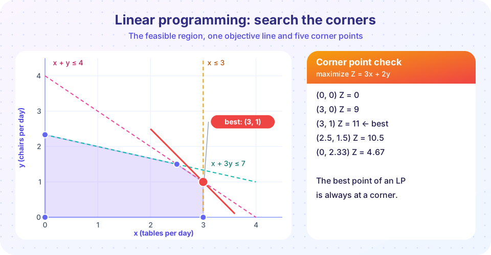
Each inequality is a half-plane, bounded by a line. The feasible region is where all the half-planes overlap: here, the polygon with corners (0, 0), (3, 0), (3, 1), (2.5, 1.5) and (0, 7/3). To find where x + y = 4 meets x + 3y = 7, subtract: 2y = 3, so y = 1.5 and x = 2.5.
Every point of the objective Z = 3x + 2y = c lies on a line of slope −3/2. Increasing c slides the line up and to the right. The last point of the polygon the line touches is the optimum. A line can only touch a polygon last at a corner (or along a whole edge if it is parallel to it), which gives the corner point theorem: if an LP has an optimum, one is at a corner.
| Corner | Z = 3x + 2y |
|---|---|
| (0, 0) | 0 |
| (3, 0) | 9 |
| (3, 1) | 11 |
| (2.5, 1.5) | 10.5 |
| (0, 7/3) | 4.67 |
The best is (3, 1) with Z = 11, that is 1,100 dollars per day. Check the constraints there: wood 3 + 1 = 4 (used up), carpentry 3 + 3 = 6 ≤ 7 (one hour spare), finishing 3 = 3 (used up). The wood and finishing constraints are binding; carpentry has a slack of 1 hour.
Shadow prices
Ask the manager's favourite question: "What is one more sheet of wood worth?" Increase the wood to 5 sheets. With the finishing limit still at 3 tables, the extra wood can only go to chairs, and carpentry allows y up to 4/3. So the new optimum is (3, 4/3) with Z = 9 + 8/3 = 11.67. The gain per sheet is 2 (hundred dollars): the shadow price of wood equals the profit of one chair batch.
But notice how it is limited. After y reaches 4/3 (using just one-third of an extra sheet) carpentry becomes binding and more wood is worthless. A shadow price is valid only within a range of the right-hand side, and sensitivity analysis reports that range. Similarly, the shadow price of the finishing limit is 1: each extra table batch could replace one chair batch (wood is tight) and earns 3 − 2 = 1 more.
Press Run (or Ctrl + Enter) to see the result here.
Program input · what you'd type while the program runs
Type the answers before you press Run, one per line. Each time the program reads a line (with input()), it gets the next line from this box.
Common misconceptions
"The optimum is wherever the objective is largest in the middle of the region." For a linear objective the middle is never best: you can always improve by moving toward the boundary.
"Round the LP answer to get the integer answer." If batches must be whole numbers, rounding can break a constraint or miss the true best integer solution. That needs integer programming.
"A shadow price is the price you should pay." It is the most the resource is worth to you, and only for a limited range.
Doing it from scratch
SciPy hides the algorithm. The corner point theorem gives a simple, if inefficient, method: intersect every pair of constraint lines, keep the feasible intersections, and evaluate the objective at each. The simplex method is a clever way of walking from corner to corner without visiting all of them.
Press Run (or Ctrl + Enter) to see the result here.
Program input · what you'd type while the program runs
Type the answers before you press Run, one per line. Each time the program reads a line (with input()), it gets the next line from this box.
How robust is the answer?
What if the profit per chair batch is uncertain? Keep the table profit at 3 and vary the chair profit c. The next plot shows the best achievable profit. It is made of straight pieces, and the optimal corner changes only at a few special values.
Press Run (or Ctrl + Enter) to see the result here.
Program input · what you'd type while the program runs
Type the answers before you press Run, one per line. Each time the program reads a line (with input()), it gets the next line from this box.
Check your understanding
Quick check · 5 questions
of 5 answered You scored / 5 · perfect!
-
1. Where does the optimum of a linear program lie?
A linear objective is maximized at a vertex of the feasible polygon, or along an edge between two optimal vertices. -
2. At the optimum (3, 1) the carpentry constraint x + 3y <= 7 gives 6. This means:
Only 6 of the 7 hours are used, so the slack is 1 hour and the constraint is not binding. -
3. What does a shadow price of 2 for wood mean?
A shadow price is the marginal value of a binding resource, valid while the same constraints stay binding. -
4. Which problem is NOT a linear program?
The product x*y is nonlinear, so that objective is not allowed in an LP. -
5. If the chair profit rises from 2 to 4 (table profit stays 3), what happens to the optimal corner?
The corner (3, 1) stays optimal only up to a chair profit of 3; above that, (2.5, 1.5) is best until the profit reaches 9.
Summary
- An LP has a linear objective and linear constraints; write variables with units first.
- The feasible region is a polygon; the optimum is at a corner.
- Binding constraints use up a resource; slack measures what is left over.
- A shadow price is the value of one extra unit of a binding resource, valid only over a range.
Track your progress
Create a free account to tick off lessons and pick up where you left off on any device.
of Mathematical Modelling lessons completed