


















Lesson 4 of 46 · Getting Started
The Python Modelling Toolkit
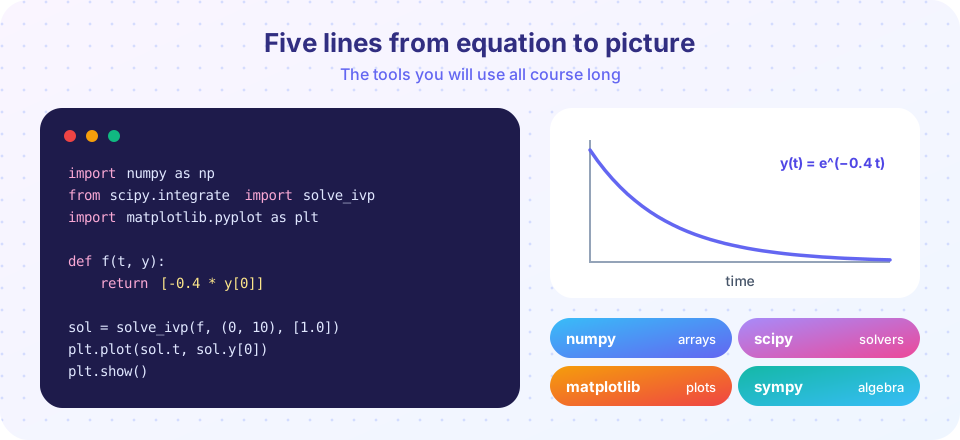
Meet the four Python libraries you will use all course: NumPy for arrays, SciPy for solvers, SymPy for algebra and Matplotlib for clear, honest plots.
A model on paper is a promise. A model in code is a machine you can switch on, poke and break. Python has become the working language of modelling because a handful of libraries turn long afternoons of arithmetic into a few lines you can read aloud. Everything here runs in your browser, so there is nothing to install.
This lesson is a guided tour. You do not need to memorize it; you will use each tool again and again in later chapters, and you can always come back.
What you will learn
- How NumPy arrays let you compute thousands of values at once
- How to simulate a model step by step and with SciPy's solver
- How SymPy checks algebra for you
- How to make a plot that actually communicates
Key terms
Array: a block of numbers that can be processed together, written np.array([...]).
Vectorized: written so that one expression works on a whole array instead of a loop over single numbers.
Euler's method: the simplest way to solve dy/dt = f(t, y) numerically: repeat y_new = y + f(t, y) · dt.
Symbolic computation: working with exact algebra (letters and formulas) rather than numbers.
Time step dt: the small interval between simulated moments.
NumPy: numbers in bulk
NumPy gives you arrays and fast operations on them. Instead of looping over every time value, you write the formula once:
t = np.linspace(0, 10, 101)   # 101 evenly spaced times from 0 to 10
y = np.exp(-0.4 * t)          # the formula applied to all 101 values
np.linspace(a, b, n) makes n evenly spaced points, np.arange(a, b, step) counts by a step, and functions such as np.exp, np.sqrt and np.log work on whole arrays. Arrays also take simple summaries: y.max(), y.sum(), y.mean().
Press Run (or Ctrl + Enter) to see the result here.
Program input · what you'd type while the program runs
Type the answers before you press Run, one per line. Each time the program reads a line (with input()), it gets the next line from this box.
Euler's method: a model as a loop
Many models say how fast something changes: dy/dt = f(t, y). You usually cannot solve that with algebra, but you can walk forward in small steps. If y is the value now, the value a short time dt later is about
y_new = y + f(t, y) · dt
That is Euler's method, named after Leonhard Euler, who described it in the 1700s. It is a simulation in its purest form: start at the initial value and keep applying the rule. Smaller steps give better answers but need more of them.
SciPy: a professional solver
For real work you rarely write Euler loops. scipy.integrate.solve_ivp picks step sizes automatically to meet an accuracy target. You give it the rate function, a time interval and a starting value:
sol = solve_ivp(lambda t, y: -0.4 * y, (0, 10), [1.0], t_eval=np.linspace(0, 10, 101))
The result sol.t holds the times and sol.y[0] the values. solve_ivp also gets the shape of fast-changing curves right with far fewer points than a naive Euler loop.
Press Run (or Ctrl + Enter) to see the result here.
Program input · what you'd type while the program runs
Type the answers before you press Run, one per line. Each time the program reads a line (with input()), it gets the next line from this box.
You should see the error shrink roughly in proportion to dt. Euler's method is first order: halve the step, halve the error. That is a general fact you can use to test your own code.
SymPy: let the computer do the algebra
SymPy works with exact formulas. It can differentiate, integrate, simplify and solve equations. This is a safety net: after solving a model by hand, check your answer symbolically.
Press Run (or Ctrl + Enter) to see the result here.
Program input · what you'd type while the program runs
Type the answers before you press Run, one per line. Each time the program reads a line (with input()), it gets the next line from this box.
Matplotlib: plots that explain
A plot is an argument, not decoration. A reader should be able to answer "what is plotted, in what units, and what should I notice?" in five seconds. A good habit list:
- Label both axes with units.
- Give the plot a title that states the message.
- Use
linewidth=2.5or more, and distinct colors. - Annotate the one feature that matters with
plt.annotate. - Start
yaxes at zero for bars, but choose a sensible range for curves.
Common misconceptions
"The solver's answer is exact." Numerical solutions are approximations controlled by tolerances. Always check one case against a known formula, as above.
"A smoother plot means a better model." Smoothness comes from how many points you plot. It says nothing about whether the model is right.
"Symbolic algebra replaces thinking." SymPy is a checker, not an oracle. You still choose the question and interpret the answer.
Try it
Now let the computer find a number you could not get by hand easily. The cooling model dT/dt = −k (T − 21) has a closed form, but pretend it did not. Use solve_ivp with an event to detect the moment the coffee reaches 60 °C.
Press Run (or Ctrl + Enter) to see the result here.
Program input · what you'd type while the program runs
Type the answers before you press Run, one per line. Each time the program reads a line (with input()), it gets the next line from this box.
Check your understanding
Quick check · 5 questions
of 5 answered You scored / 5 · perfect!
-
1. What does np.linspace(0, 10, 101) create?
linspace(a, b, n) gives n evenly spaced values that start at a and end at b. -
2. In Euler's method, what happens to the error when you halve the time step?
Euler's method is first order, so the error is roughly proportional to the step size. -
3. Which library would you use to check a formula symbolically?
SymPy manipulates exact algebraic expressions: differentiate, simplify, solve. -
4. Why call solve_ivp instead of writing your own Euler loop for a serious problem?
Adaptive step control gives accurate results with few steps and fewer opportunities for mistakes. -
5. A good plot of a model result should:
Readers should know what is plotted, in what units, and what to notice.
Summary
- NumPy computes with whole arrays at once;
linspace,expand boolean filtering cover most needs. - Euler's method turns
dy/dt = f(t, y)into a loop; its error is proportional to the step. solve_ivpis the professional solver and can detect events such as "reaches 60 °C".- SymPy checks algebra and solves exact equations.
- Good plots have labeled axes with units, a message title and one clear annotation.
Next: Chapter 1 Review
Track your progress
Create a free account to tick off lessons and pick up where you left off on any device.
of Mathematical Modelling lessons completed