


















Lesson 30 of 46 · Optimization Models
Chapter 6 review: optimization models
Review calculus optimization, linear programming and gradient descent with a summary poster, a method-choice table, runnable checks and a ten-question quiz.
You can now pose a question as "choose these variables, obey these limits, optimize this goal" and attack it with three different tools. This page gathers the chapter on one poster, helps you choose a method, lets you check one problem with four methods at once, and ends with a ten-question quiz.
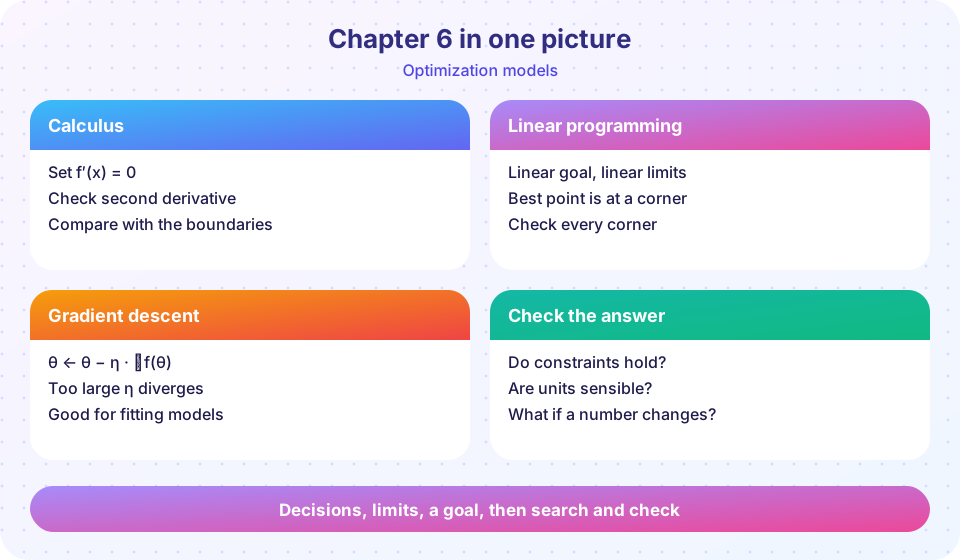
Which method should I use?
| Situation | Method | Why |
|---|---|---|
| One or two variables, smooth formula | Calculus: set f′ = 0, check |
Exact answer, shows structure |
| Many variables, everything linear | Linear programming (simplex, HiGHS) | Corner point theorem, shadow prices |
| Many variables, smooth but complicated | Gradient descent or scipy.optimize.minimize |
Needs only gradients or values |
| Whole numbers required | Integer programming | LP rounding can fail |
| Many local minima | Multi-start or global search | A single start may trap you |
The checking habit
An optimal answer is only as good as the model, so spend a minute on three checks:
- Feasibility. Plug the answer back into every constraint.
- Reasonableness. Are units and sizes plausible? A can 7.5 cm tall is realistic; one 7.5 m tall is not.
- Sensitivity. Change a number by 10 percent. If the answer jumps, you need better data for that number. If it barely moves, relax.
Try it
The same can problem, four ways. They should agree to several digits.
Press Run (or Ctrl + Enter) to see the result here.
Program input · what you'd type while the program runs
Type the answers before you press Run, one per line. Each time the program reads a line (with input()), it gets the next line from this box.
Next, a feasibility checker for the workshop linear program from the previous lesson. It is the first of the three checks in practice.
Press Run (or Ctrl + Enter) to see the result here.
Program input · what you'd type while the program runs
Type the answers before you press Run, one per line. Each time the program reads a line (with input()), it gets the next line from this box.
Check your understanding
Quick check · 10 questions
of 10 answered You scored / 10 · perfect!
-
1. A fence problem gives 2x + 2y = 40. What is this equation called?
It limits the allowed choices of x and y, so it is a constraint. -
2. After setting f'(x) = 0, why do you still check the endpoints?
On a closed interval the largest or smallest value can occur at an end. -
3. For a cylinder of fixed volume with minimum surface area, h/r equals:
The optimum has height equal to the diameter, so h = 2r. -
4. In a linear program, where is the optimum found?
By the corner point theorem. -
5. A binding constraint is one that:
A binding constraint is fully used at the optimum. -
6. A shadow price of 2 for wood is valid:
When another constraint becomes binding, the value of extra wood changes. -
7. In gradient descent, the update is:
We move against the gradient to go downhill. -
8. For f = x^2 + 5y^2, the largest stable learning rate is below:
The y-factor |1 - 10 eta| must be less than 1, so eta < 0.2. -
9. Why can gradient descent end at different answers from different starts?
In a non-convex landscape each start slides into the nearest valley. -
10. Changing a parameter by 10 percent moves your optimum a lot. What does that tell you?
Sensitivity tells you which inputs deserve the best data.
Summary
- Optimization model = decision variables + constraints + one objective.
- Calculus for smooth one- or two-variable problems, LP for linear ones, descent for the rest.
- Always check feasibility, reasonableness and sensitivity.
- Shadow prices and learning-rate limits are the two numbers to remember from this chapter.
Track your progress
Create a free account to tick off lessons and pick up where you left off on any device.
of Mathematical Modelling lessons completed