


















Lesson 33 of 49 · Transcriptomics and Expression
Chapter 6 Review: Transcriptomics and Expression
Review the RNA-seq analysis path from counts to normalization, testing, FDR control, heatmaps and enrichment, with a recap table, a checklist and a ten-question quiz.
This chapter followed the logic of an RNA-seq study: count reads per gene, make the counts comparable, test every gene, control the false discoveries, and then look for patterns and pathways. Each step has a standard tool and a standard trap. This review lays them side by side so you can see the whole path in one place, and then practices the thinking you need when a result looks too good, or too strange.
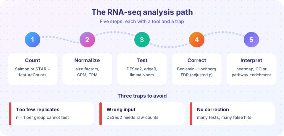
The chapter in one table
| Step | Question | Typical tools | Remember |
|---|---|---|---|
| Count (overview) | How many reads per gene? | STAR + featureCounts, Salmon, kallisto | Matrix of genes by samples; raw integer counts |
| Normalize (lesson) | Are samples comparable? | size factors, TMM, TPM, VST | Depth, length, composition; TPM sums to 10^6 |
| Test (lesson) | Which genes changed? | DESeq2, edgeR, limma-voom | Var = mu + alpha * mu^2; LFC is effect size |
| Correct | How many are false? | Benjamini-Hochberg | FDR 5% means about 5% of the list is wrong |
| Explore and interpret (lesson) | What do changes mean? | PCA, heatmaps, GO/KEGG, GSEA | Universe and correction change enrichment |
Ideas that connect the steps
Relative, not absolute. RNA-seq shares a fixed number of reads among all genes. Normalization exists because a change in one gene's share affects the others. Whenever a result is surprising, ask whether composition or depth could explain it.
Replicates carry the statistics. The dispersion term in the negative binomial model does not shrink as you sequence deeper. Only independent biological replicates reduce uncertainty about a gene's mean, which is why three per group is the floor and not the target.
Two numbers, always together. A fold change without a measure of evidence is a guess, and a p-value without an effect size is trivia. The volcano plot is useful because it makes you look at both at once.
Thresholds are choices. The cut-offs padj < 0.05 and |LFC| > 1 are conventions, not laws. The enrichment universe, the minimum count filter, and the linkage method are also choices that change the outcome. Record them, and check that your conclusion survives reasonable alternatives.
Statistics proposes, biology disposes. A significant gene list and an enriched pathway are hypotheses. Orthogonal validation (qPCR of a few genes, an independent cohort, a knockout) is what turns them into findings.
A reproducible checklist
- Design: biological replicates per group (at least three), batches recorded and balanced across conditions.
- Counts: strandedness set correctly, annotation release recorded, library sizes and percent assigned reads look similar across samples.
- Exploration: PCA and sample distances show replicates together and no unexplained batch structure.
- Testing: raw counts into DESeq2 or edgeR with the right design formula; the p-value histogram looks flat with a spike near zero.
- Reporting: both LFC (preferably shrunken) and adjusted p-value, the filter and thresholds stated, versions of tools and annotation recorded.
Worked example: when everything is "down"
A student runs a comparison and finds that 3,000 genes are significantly down in the treated samples but only 150 are up. Her treatment is a drug that blocks one transcription factor. Is it plausible that thousands of genes truly fell?
Maybe, but check the normalization before the biology. If the treatment induces a handful of genes to very high levels (an immune response can do this), those genes consume a large share of reads, and a method that scales by total counts will make everything else look lower. The median-of-ratios method or TMM would have handled this, so first confirm which size factors she used, and compare normalized count distributions between samples. Second, plot the MA plot: with a good normalization the bulk of genes is centred on zero, and a cloud shifted below zero is a red flag. Third, look at a few spike-in or housekeeping-like genes if the experiment has them.
If the cloud centres correctly after robust normalization and 3,000 genes still go down, the finding might be real, a broad shutdown caused by the drug. The skill is not to know the answer in advance, but to order the questions: normalization and design first, interpretation last.
Three small studies, three decisions
The same toolbox gives different advice depending on the study, which is why recipes alone are not enough.
A drug-response study with eight mice per group. There is plenty of power, so a stricter cut-off such as |LFC| > 1 with padj < 0.01 keeps the list short and interpretable. Spend your effort on the batch design: if the treated mice were housed in one cage and the controls in another, cage and treatment are confounded, and no statistics can separate them.
A rare-tissue study with three samples per group. Power is low, so many true changes will not reach significance. Resist the urge to relax the threshold until things appear. Instead report the effect sizes with their uncertainty, use shrunken fold changes for ranking, and use a rank-based method such as GSEA, which can detect coordinated modest shifts that no single gene proves.
A time-course with five time points. A simple two-group comparison is the wrong tool. Use a design that models time (for example a likelihood ratio test against a reduced model), and cluster genes by their trajectories so that "rises then falls" patterns become visible.
In each case, the decision comes from asking what question the data can actually answer, then choosing the model, the correction and the visualization to match. That habit transfers to every dataset you will meet.
Try it
The first example prints a table of how many genes pass at different FDR cut-offs for simulated p-values, showing the cost of stricter control. The second is an interactive Benjamini-Hochberg plot: move the slider to change the FDR level and see which sorted p-values fall under the line.
Press Run (or Ctrl + Enter) to see the result here.
Program input · what you'd type while the program runs
Type the answers before you press Run, one per line. Each time the program reads a line (with input()), it gets the next line from this box.
Check your understanding
Quick check · 9 questions
of 9 answered You scored / 9 · perfect!
-
1. Which input does DESeq2 expect for its statistical test?
DESeq2 models raw counts with a negative binomial distribution and applies size factors internally. -
2. A gene goes from a mean normalized count of 30 to 120. Its log2 fold change is:
120 / 30 = 4, and log2(4) = 2. -
3. Which statement about TPM is true?
TPM divides by length and rescales each sample to 1,000,000, but it is still a relative measure. -
4. With m = 20 tests and q = 0.05, what threshold must the smallest p-value (rank 1) pass in BH?
(1 / 20) * 0.05 = 0.0025. -
5. Three replicates per group were sequenced twice each (six libraries per group). What did you gain?
Repeating the sequencing of the same RNA addresses technical noise, which is small compared with biological variation. -
6. What is the main role of the background gene set (universe) in enrichment analysis?
The expected overlap is computed against the genes that could have been detected. -
7. In a PCA, replicates of the same condition lie far apart but samples from the same day cluster together. The best explanation is:
Grouping by processing day points at a batch effect, which must be modelled. -
8. What does the BH adjusted p-value of 0.03 for a gene mean?
An adjusted p-value is the lowest FDR at which the gene would still be called. -
9. Why is a large fold change alone not enough to call a gene differentially expressed?
Low counts are noisy, so evidence (a p-value from replicates) must accompany the effect size.
Summary
- The path is count, normalize, test, correct, interpret; each step has a standard tool and a standard trap.
- Raw counts go into count-based tests; TPM and log-CPM are for display and within-sample comparison.
- Replicates, design with batch, and robust normalization matter more than software choice.
- Report effect size and adjusted p-value together, and state every threshold and database version.
- Enrichment and clustering suggest hypotheses that need independent validation.
Track your progress
Create a free account to tick off lessons and pick up where you left off on any device.
of Bioinformatics lessons completed