


















Lesson 29 of 49 · Transcriptomics and Expression
Chapter 6 Overview: Transcriptomics and Expression
Get the big picture of RNA-seq: what it measures, how libraries are made, how reads become a count matrix, and how groups are compared statistically.
Every cell in your body carries nearly the same DNA, yet a neuron and a liver cell behave very differently. The difference lies in which genes are switched on, and by how much. The set of RNA molecules a cell is making at a given moment is its transcriptome, and RNA-seq is the technique that measures it by sequencing.
Where the previous chapter asked "how does this genome differ from the reference?", this chapter asks "which genes are more active in condition B than in condition A?". The data are still reads, but the unit of analysis changes: instead of positions, we count reads per gene, and instead of genotypes, we test for changes in expression.
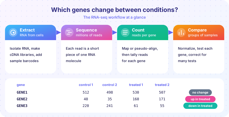
What you will learn
- What RNA-seq measures and which choices in the lab shape the data.
- How reads become a gene-by-sample count matrix.
- Why replicates, normalization and multiple-testing correction are not optional.
- How the chapter's lessons fit together into one analysis.
Key terms
Transcriptome: all RNA molecules present in a sample at one time.
Count matrix: a table with one row per gene, one column per sample, and the number of reads assigned to each gene as the entries.
Differential expression (DE): a statistically supported difference in a gene's expression between groups.
Replicate: an independent biological sample of the same condition.
Library: the prepared collection of cDNA fragments that goes into the sequencer.
What RNA-seq measures
The cell's DNA is transcribed into RNA. Most of the RNA by mass (the large majority) is ribosomal RNA, which is rarely the object of study. The remainder includes messenger RNA (mRNA) that encodes proteins, and a wide variety of non-coding RNAs. RNA-seq proceeds in steps:
- Extract RNA from cells or tissue, and check its integrity.
- Enrich what you want. Poly-A selection captures mature mRNA by its tail. rRNA depletion removes ribosomal RNA instead, which keeps non-coding RNA and works for bacteria (which lack poly-A tails) and degraded samples.
- Convert to cDNA, fragment, attach adapters and barcodes, and amplify to make the library.
- Sequence to typically 20 to 30 million reads per sample for a standard bulk differential-expression experiment.
- Quantify how many reads came from each gene, then analyze.
A key limitation: the sequencer reports relative abundance. If one gene becomes extremely abundant, it takes up a larger share of the reads and the share of every other gene shrinks, even if their absolute amounts did not change. Much of the statistics in this chapter exists to handle that fact sensibly.
Two ways to get counts
Map, then count. A splice-aware mapper such as STAR or HISAT2 aligns reads to the genome, allowing a read to jump across an intron (the N operation in a CIGAR string from the previous chapter). A counting tool such as featureCounts or HTSeq then tallies reads overlapping each gene in an annotation file (GTF).
Pseudo-alignment. Salmon and kallisto skip full alignment: they work out which transcripts each read is compatible with and estimate transcript abundance statistically. They are very fast, handle reads that fit several isoforms gracefully, and the estimates are summarized to gene level with the tximport package.
Either route ends in the same object: the count matrix. Most statistical tools for differential expression (DESeq2, edgeR) expect raw, un-normalized integer counts, a detail that matters in lesson 2.
Design the experiment
Good design cannot be fixed later
Get the counts
Rows are genes, columns are samples
Compare the groups
A volcano plot shows the result
Make sense of it
Statistics suggests, biology confirms
Design matters more than software
Biological variation between individuals, plates, or days is usually bigger than the technical noise of sequencing. That is why the number of biological replicates is the main driver of statistical power. Three per group is a common minimum; more is better when the effects are small. Technical replicates (sequencing the same RNA twice) do not substitute for biological ones.
Also plan for batch effects: if all control samples are processed on Monday and all treated samples on Tuesday, you cannot tell treatment from day. Randomize samples across batches, record the batch for every sample, and include it in the statistical model. Single-cell RNA-seq (for example with 10x Genomics chips and unique molecular identifiers) extends the idea to thousands of individual cells, but the bulk workflow here teaches the concepts that single-cell methods build on.
The annotation: how reads become genes
A counting tool needs to know where genes are. That knowledge comes from an annotation file, most often GTF or GFF3, a tab-separated table with one line per feature: the sequence name, the source, the feature type (gene, transcript, exon, CDS), start and end, strand, and a column of attributes such as the gene identifier and name. Counting at the gene level means summing reads that overlap any exon of a gene. Annotation versions matter as much as reference versions: Ensembl and GENCODE release new annotations several times a year, gene identifiers like ENSG00000139618 are stable while gene symbols such as BRCA2 can change, and two analyses using different releases can disagree about a gene's very existence. Record the release number.
Quality checks specific to RNA-seq
Beyond the FASTQ checks of the previous chapter, an RNA-seq project looks at a few extra things:
- The fraction of reads mapping to exons. DNA contamination or intron-retaining pre-mRNA shows up as reads in introns and intergenic regions.
- Ribosomal RNA content. High rRNA after depletion means the depletion failed and the useful read depth is much lower than the nominal one.
- Gene body coverage. With poly-A selection, coverage often leans towards the 3' end when the RNA was degraded.
- Sample relationships. Replicates of one condition should resemble each other more than samples of another condition, which a principal component plot shows quickly. A sample that sits alone is either biology or a mix-up, and you must find out which.
- Strandedness. Modern kits record which strand the RNA came from, and the counting step must be told how, or reads from antisense transcripts get assigned to the wrong gene.
What each lesson covers
| Lesson | What you will do |
|---|---|
| Counts and Normalization | Compare CPM, TPM and size factors; see why raw counts mislead. |
| Differential Expression | Test every gene, adjust p-values with Benjamini-Hochberg, read a volcano plot. |
| Clustering, Heatmaps and Enrichment | Group genes and samples, then ask which pathways are over-represented. |
| Chapter Review | Tie the pipeline together and practice pitfalls. |
Try it
The first example turns the counts from the figure into counts per million, given the library sizes of the four samples (the numbers are illustrative). The second shows why RNA-seq counts are not simply Poisson: biological replicates vary more than chance alone predicts.
Press Run (or Ctrl + Enter) to see the result here.
Program input · what you'd type while the program runs
Type the answers before you press Run, one per line. Each time the program reads a line (with input()), it gets the next line from this box.
Press Run (or Ctrl + Enter) to see the result here.
Program input · what you'd type while the program runs
Type the answers before you press Run, one per line. Each time the program reads a line (with input()), it gets the next line from this box.
Check your understanding
Quick check · 4 questions
of 4 answered You scored / 4 · perfect!
-
1. What are the rows and columns of an RNA-seq count matrix?
Each entry is the number of reads assigned to one gene in one sample. -
2. Why is poly-A selection unsuitable for bacterial RNA?
Poly-A selection captures RNAs with poly-A tails, which are typical of eukaryotic mRNA; bacteria usually need rRNA depletion. -
3. Which design choice most improves statistical power in a bulk RNA-seq experiment?
Biological variation dominates, so independent biological replicates help most. -
4. What does it mean that RNA-seq measures relative abundance?
The sequencer samples a fixed number of reads, so shares shift when some genes become very abundant.
Summary
- RNA-seq counts reads per gene to estimate which genes are active; it measures relative abundance.
- The path is extract, enrich (poly-A or rRNA depletion), build libraries, sequence, then map or pseudo-align and count.
- Biological replicates and randomized batches matter more than any software choice.
- The next lessons cover normalization, differential-expression testing with false-discovery control, and interpretation with clustering and enrichment.
Next: Counts and Normalization
Track your progress
Create a free account to tick off lessons and pick up where you left off on any device.
of Bioinformatics lessons completed