


















Lesson 32 of 49 · Transcriptomics and Expression
Clustering, Heatmaps and Pathway Enrichment
Learn to explore expression data with PCA, hierarchical clustering and heatmaps, and to interpret gene lists with over-representation analysis and GSEA.
A differential expression table can hold a few hundred genes. Staring at that list rarely tells you the story. Two kinds of analysis help. Exploratory analysis (PCA, clustering and heatmaps) shows how samples and genes group, and whether the data are healthy. Enrichment analysis asks whether the genes you found share a function more often than chance would predict, which turns a list of names into biological themes.
Both are easy to run and easy to over-interpret. This lesson explains how they work, what the pictures can and cannot show, and which small decisions (scaling, background gene set, correction) change the answer.
What you will learn
- How PCA and sample-distance plots reveal data quality and batch effects.
- How hierarchical clustering and heatmaps are built, including scaling by gene.
- How over-representation analysis uses the hypergeometric test, and what the background means.
- How GSEA differs, and why enrichment results need correction and caution.
Key terms
PCA (principal component analysis): a way to project many-dimensional data onto a few axes that capture the most variance.
Hierarchical clustering: building a tree by repeatedly merging the two most similar items.
z-score: (value - gene mean) / gene standard deviation; puts every gene on a common scale.
Gene Ontology (GO): a curated vocabulary of biological processes, molecular functions and cellular components, with genes annotated to terms.
Background (universe): the set of genes that could have been found; the reference for "expected by chance".
Start with the samples: PCA
Before looking at any gene, look at the samples. PCA finds the direction in gene-expression space along which the samples vary the most (PC1), then the next most (PC2) at right angles, and so on. Plotting samples on PC1 versus PC2 shows the main structure in the data in one picture. You run PCA on normalized and variance-stabilized values (see the normalization lesson), usually on the few thousand most variable genes.
What a healthy experiment looks like: replicates of the same condition sit close together, and the conditions separate along PC1 or PC2. What to worry about:
- A single sample far from its replicates: a failed library, a mislabel or genuine biology.
- Samples that separate by batch, extraction date or sequencing lane rather than by condition. The effect must go into the statistical model, and if conditions and batches are perfectly confounded, no analysis can separate them.
- A sample that clusters with the wrong group, which could be a swap.
PCA axes are labelled with the percentage of variance explained. If PC1 explains 60% and separates your conditions, the biology dominates the data; if the separating axis is PC4 at 3%, the signal is subtle.
Clustering genes and drawing a heatmap
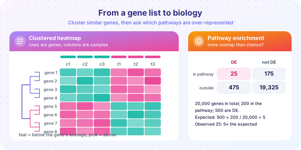
A heatmap shows a matrix as colors: rows are genes, columns are samples. On its own the figure is just a rainbow; its value comes from ordering the rows and columns so similar ones are neighbors. That ordering comes from clustering.
The usual recipe:
- Choose the genes. All 20,000 would be noise. Use the differentially expressed genes, or the top few thousand most variable ones.
- Scale each gene. Convert each row to a z-score so a gene's pattern, not its absolute level, drives the picture. Otherwise highly expressed genes dominate everything. A color then means "above or below this gene's own average".
- Measure distance between genes. Euclidean distance on z-scores, or
1 - correlation, is the standard choice. Two genes that rise and fall together get a small distance even if one is 100 times more abundant. - Merge hierarchically. Start with each gene in its own cluster and keep joining the two closest clusters. The definition of "closest between clusters" is the linkage: complete (largest pairwise distance), average, or Ward (smallest increase in variance). The resulting tree is the dendrogram.
- Cut the tree at a height to get a chosen number of clusters, or let the picture speak.
K-means is the alternative: you pick the number of clusters k and it assigns each gene to the nearest of k centres, iterating until stable. It is fast but needs k in advance, and can give different answers from different random starts.
Remember that clustering always returns clusters, even for pure noise. A tidy block pattern is a hypothesis to check with biology, not a proof. Also keep the color scale honest: a symmetrical scale around zero, clearly labeled, and annotation bars for condition and batch above the columns.
From a gene list to biology: over-representation analysis
Suppose 500 genes are up in treated samples. Are they just a random handful of the genome, or do they hold a suspicious number of, say, "inflammatory response" genes? Gene sets come from curated databases:
- Gene Ontology (GO) has three branches (biological process, molecular function, cellular component). Terms form a hierarchy: a gene annotated to a specific term inherits all its parents.
- KEGG and Reactome contain curated pathways.
- MSigDB collects many sets, including the 50 "Hallmark" sets that summarize well-defined processes.
Over-representation analysis (ORA) asks, for each set, whether your list overlaps it more than expected. Build a 2 by 2 table as in the figure:
| in your DE list | not in the list | |
|---|---|---|
| in the pathway | 25 | 175 |
| not in the pathway | 475 | 19,325 |
With 20,000 genes in the universe, a 200-gene pathway and a 500-gene DE list, you would expect 500 * 200 / 20,000 = 5 genes in the overlap by chance. You observe 25, a fold enrichment of 5. The probability of seeing 25 or more by chance follows the hypergeometric distribution (equivalent to a one-sided Fisher exact test), and here it is extremely small.
Three decisions affect the answer:
- The universe. It should be the genes that were measurable in your experiment (expressed above the filter), not the whole genome. Using the wrong background inflates enrichment for tissue-specific terms.
- Multiple testing. You test thousands of gene sets, so correct the p-values (BH) as you did for genes.
- Redundancy. GO terms overlap heavily, so ten significant terms may be one finding. Tools that merge similar terms or visualize networks help.
GSEA: no cutoff needed
ORA depends on an arbitrary cutoff for the list. Gene set enrichment analysis (GSEA), introduced by Subramanian and colleagues in 2005, avoids it. You rank all genes by a statistic (for example the signed test statistic or log fold change). For each set, GSEA walks down the ranked list: each time it meets a member of the set, the running score goes up; each time it meets a non-member, it goes down by a smaller amount. The maximum deviation from zero is the enrichment score. Normalizing by permutation gives a normalized enrichment score (NES) and an FDR. A set whose members cluster at the top (or bottom) of the ranking is enriched even if none of them crosses a significance threshold on its own. This makes GSEA good at catching coordinated, modest changes.
Pitfalls
- Annotation bias. Well-studied genes have many annotations, so they appear in many significant sets; poorly studied genes are invisible to enrichment.
- Identifier mapping. Converting between Ensembl IDs, gene symbols and Entrez IDs loses or duplicates genes. Report how many mapped.
- Interpretation. Enrichment suggests a theme; it does not prove the pathway is active. Test the key genes in the lab or with an independent dataset.
Common misconceptions
"The clusters in my heatmap are real groups." Hierarchical clustering produces a tree for any data; check stability (different linkage, resampling) and biological meaning.
"A significant GO term means the pathway is switched on." It means your genes overlap the set more than chance predicts, subject to the background and correction choices.
"PCA shows differential expression." PCA shows the largest sources of variation, which may be batch effects. It describes the data; it does not test hypotheses.
Try it
First, cluster simulated genes and draw a heatmap with a dendrogram order. Second, run an enrichment test for the numbers in the figure and then across several pathways with correction. Third, draw a PCA of samples to see condition and batch effects.
Press Run (or Ctrl + Enter) to see the result here.
Program input · what you'd type while the program runs
Type the answers before you press Run, one per line. Each time the program reads a line (with input()), it gets the next line from this box.
Press Run (or Ctrl + Enter) to see the result here.
Program input · what you'd type while the program runs
Type the answers before you press Run, one per line. Each time the program reads a line (with input()), it gets the next line from this box.
Press Run (or Ctrl + Enter) to see the result here.
Program input · what you'd type while the program runs
Type the answers before you press Run, one per line. Each time the program reads a line (with input()), it gets the next line from this box.
Check your understanding
Quick check · 5 questions
of 5 answered You scored / 5 · perfect!
-
1. Why do we usually z-score each gene before drawing a heatmap?
Z-scoring puts all genes on a common scale so a highly expressed gene does not dominate. -
2. A DE list has 500 genes out of 20,000. A pathway has 200 genes. How many overlaps do you expect by chance?
Expected overlap is 500 * 200 / 20,000 = 5. -
3. What is the problem with using all genes in the genome as the background when only 12,000 genes were expressed in your experiment?
Genes that could never be detected should not count as chances to overlap; the universe should be the measurable genes. -
4. How does GSEA differ from over-representation analysis?
GSEA walks down a ranked list of all genes and detects coordinated shifts of a set's members. -
5. In a PCA plot, samples of one condition separate along PC1, which explains 55% of variance. What does this suggest?
A large axis that tracks the condition means biology dominates; check other PCs for batch.
Summary
- Explore samples first with PCA and clustering; look for outliers, swaps and batch effects.
- For heatmaps choose informative genes, z-score each row, pick a distance and linkage, and annotate samples with condition and batch.
- Clustering always returns clusters; verify patterns before believing them.
- Over-representation analysis tests a gene list against sets with the hypergeometric (Fisher) test; the universe and multiple-testing correction matter.
- GSEA uses all ranked genes and finds coordinated modest changes; enrichment suggests themes that need validation.
Track your progress
Create a free account to tick off lessons and pick up where you left off on any device.
of Bioinformatics lessons completed