


















Lesson 19 of 49 · Phylogenetics
Distances and UPGMA
Turn an alignment into evolutionary distances with p-distance and the Jukes-Cantor correction, then build a tree by UPGMA clustering, with Python code and the molecular-clock caveat.
The simplest way to build a tree is to measure how different each pair of sequences is, put those numbers into a table, and let a clustering procedure turn the table into a tree. These distance methods are fast, easy to understand and good enough for many jobs. They also teach the central difficulty of molecular phylogenetics: the differences you can count are only a lower bound on the changes that really happened. This lesson shows how to correct for that and then builds a tree with UPGMA, the oldest clustering method.
What you will learn
- How to compute the p-distance and why it underestimates true divergence.
- The Jukes-Cantor correction, its assumptions and where it breaks (saturation).
- The UPGMA algorithm step by step, with the formula for averaging distances.
- What a molecular clock is and why UPGMA can go wrong without one.
Key terms
- p-distance: the fraction of aligned sites that differ between two sequences.
- Multiple hits: several substitutions at the same site, which hide each other.
- Saturation: the point where more evolution no longer increases the observed difference.
- Molecular clock: the assumption that substitutions accumulate at a roughly constant rate.
- Ultrametric tree: a rooted tree in which every leaf is the same distance from the root.
From an alignment to a distance
Start with an alignment of two sequences of length L (ignoring gaps for now). If D sites differ, the p-distance is p = D / L. For two 200-base sequences that differ at 30 sites, p = 0.15. Because we want a distance that grows in proportion to the time since the sequences diverged, the p-distance would be ideal, if only each substitution left a visible trace.
It does not. A site can mutate from A to G and later from G to T, which looks like a single change from A to T. It can mutate from A to G and back to A, which looks like no change at all. These multiple hits accumulate as sequences diverge, so the observed difference lags behind the true number of substitutions. For random DNA two unrelated sequences already agree at about one quarter of sites by chance, so the p-distance can never exceed 0.75 however old the split.
The Jukes-Cantor correction
Thomas Jukes and Charles Cantor (1969) proposed the simplest model that lets us undo this effect. Assume every site changes at the same rate and that any base is equally likely to turn into any of the three others. Under this model the expected number of substitutions per site since the divergence, d, relates to the observed p-distance by
d = -(3/4) * ln(1 - (4/3) * p)
For small p, d is close to p (a few differences are mostly single hits). As p approaches 0.75, the logarithm explodes and d becomes infinite, which is the mathematics of saturation: at 0.75 the sequences are as different as random ones and carry no further signal about time. A p of 0.30 corrects to d = -0.75 ln(0.6) = 0.383, noticeably larger. Real data are more complicated, and richer models exist. Kimura's two-parameter model (K2P) allows transitions and transversions to differ in rate; Tamura-Nei and the GTR model also let base frequencies and each substitution type vary. For proteins one uses the Poisson correction d = -ln(1 - p) or distances based on a substitution matrix such as JTT or LG. The principle remains the same: estimate the number of substitutions, not the number of visible differences.
Distances computed this way form a symmetric matrix with zeros on the diagonal. Whenever possible, compute them from a well-curated alignment, because a distance is only as good as the columns that feed it.
UPGMA: clustering by average distance
UPGMA stands for Unweighted Pair Group Method with Arithmetic mean. It was introduced by Sokal and Michener in 1958 for classifying organisms by similarity, and it is a special case of average-linkage clustering. The procedure is short:
- Treat each sequence as its own cluster. Set the height of every leaf to 0.
- Find the two clusters i and j with the smallest distance
d(i, j). - Merge them into a new cluster. Place the new node at height
d(i, j) / 2and give each of the two joined branches the length from its child's height to the new height. - Compute the distance from the new cluster to every other cluster k as the size-weighted average
d(k, ij) = (n_i * d(k, i) + n_j * d(k, j)) / (n_i + n_j), wherenis the number of original sequences in a cluster. - Repeat from step 2 until one cluster remains. It is the root.
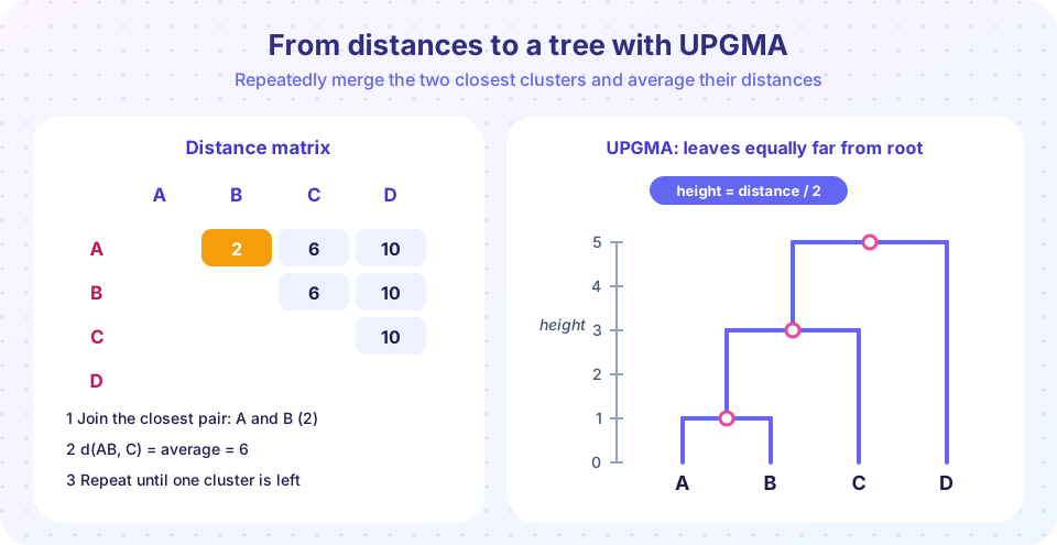
In the example on this page the matrix has distances AB = 2, AC = 6, AD = 10, BC = 6, BD = 10 and CD = 10. The smallest value, 2, joins A and B at height 1. The distance from C to the cluster (A,B) is the average of 6 and 6, which is 6; C joins at height 3. The distance from D to the combined cluster (A,B,C) is 10, and D joins at height 5. The result is a rooted tree where all leaves sit at the same distance from the root.
The molecular-clock assumption
UPGMA implicitly assumes that substitutions accumulate at the same rate along every lineage. If so, the distance between two leaves is proportional to twice the time since their common ancestor, which is why the tree is ultrametric and heights equal half the distance. When rates are equal ("clock-like") UPGMA recovers the correct tree from correct distances. When rates differ, a fast-evolving lineage looks more distant from everything than it really is, and UPGMA may place it incorrectly, typically pulling it to the base of the tree. This failing is serious for real data, where rates vary between genes, organisms and even sites. That is the motivation for neighbor-joining in the next lesson, which does not assume a clock. UPGMA remains useful when a clock is plausible, such as for closely related sequences from a single outbreak or population, and as a quick method to build guide trees for multiple alignment.
Representing the tree: Newick
Programs exchange trees in the Newick format, which uses nested parentheses and colons for branch lengths. The tree above, with branch lengths from the heights, is written (((A:1,B:1):2,C:3):2,D:5);. The semicolon ends the tree. You will see it again in the bootstrap lesson.
Common misconceptions
- "The p-distance is the evolutionary distance." It underestimates the true number of substitutions, increasingly so for distant sequences.
- "UPGMA reveals the order in which species diverged under any circumstances." It does so only if rates are roughly constant.
- "A bigger distance always means older." At saturation, the observed difference stops growing.
- "The root position is data." The UPGMA root is a consequence of the clock assumption, not something observed.
Try it
Press Run (or Ctrl + Enter) to see the result here.
Program input · what you'd type while the program runs
Type the answers before you press Run, one per line. Each time the program reads a line (with input()), it gets the next line from this box.
Press Run (or Ctrl + Enter) to see the result here.
Program input · what you'd type while the program runs
Type the answers before you press Run, one per line. Each time the program reads a line (with input()), it gets the next line from this box.
Check your understanding
Quick check · 5 questions
of 5 answered You scored / 5 · perfect!
-
1. Why does the p-distance underestimate the number of substitutions between distant sequences?
Multiple hits, including back mutations, reduce the observed differences relative to the real number of changes. -
2. What is the Jukes-Cantor distance for p = 0 ?
d = -0.75 ln(1 - 0) = 0. -
3. In UPGMA, what is the height of a node joining clusters at distance 8?
Node height is half the distance, because both branches span the time since the common ancestor. -
4. Clusters of sizes 2 and 1 are at distances 6 and 9 from a third cluster. What is the UPGMA distance after merging them?
(2 x 6 + 1 x 9) / 3 = 7. -
5. What goes wrong with UPGMA when evolutionary rates differ between lineages?
UPGMA assumes a clock, so rate differences distort the tree.
Summary
- Observed p-distances underestimate divergence; Jukes-Cantor corrects with
d = -3/4 ln(1 - 4p/3)and fails at saturation (p = 0.75). - UPGMA repeatedly merges the closest clusters, sets heights to half the distance and averages distances by cluster size.
- It assumes a molecular clock; without one, use neighbor-joining or character-based methods.
- Newick is the standard text format for trees.
Next: Neighbor-joining
Track your progress
Create a free account to tick off lessons and pick up where you left off on any device.
of Bioinformatics lessons completed