


















Lesson 24 of 49 · Genomics Pipelines
Chapter 5 Overview: Genomics Pipelines
See the whole short-read genomics pipeline at a glance: sequencing, FASTQ, mapping, BAM, variant calling, VCF and annotation, with the numbers behind each step.
A single human genome has about 3.1 billion letters. No instrument can read them in one piece. Instead, a sequencer reads millions of short fragments, and software has to work out where each fragment came from and how the person's DNA differs from a reference. That software chain is a genomics pipeline, and this chapter walks you through it from the first file to the final list of variants.
Almost every genomics project, from a rare-disease diagnosis to a study of antibiotic resistance in bacteria, uses the same skeleton. The tools change from year to year, but the files and the ideas stay remarkably stable. Learn the skeleton once and you can read any new paper's methods section.
What you will learn
- The four stages of a short-read pipeline and the file each one produces.
- Why sequencing depth, read length and quality decide what you can find.
- How to read a FASTQ, SAM and VCF line without a manual.
- Which checks catch problems early, before they reach your results.
Key terms
Read: one sequenced fragment of DNA, usually 50 to 300 bases long for short-read machines.
Reference genome: an agreed sequence (such as GRCh38 for humans) that reads are compared against.
Coverage or depth: the average number of reads that overlap each position of the genome.
Variant: a position where the sample differs from the reference.
Pipeline: a chain of programs where each output file is the next program's input.
The big picture in four stages
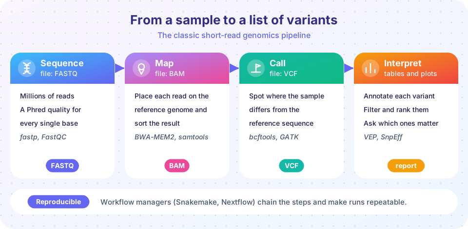
Open any lab's analysis folder and you will find the same four layers of files.
- Sequencing produces FASTQ files: text files holding reads and one quality score for every base.
- Mapping (also called alignment) places each read on the reference and writes a BAM file, a compressed table of alignments.
- Variant calling looks down the stacked reads at every position and writes a VCF file of the places where the sample differs.
- Interpretation annotates each variant with the gene it hits, its predicted effect and how common it is in population databases, then filters and ranks them.
Stage 1: Sequence
Output: FASTQ
Stage 2: Map
Output: BAM
Stage 3: Call
Output: VCF
Stage 4: Interpret
Output: a short list
Three numbers that shape every project
Read length. Short-read platforms such as Illumina typically produce reads of 100 to 150 bases, usually in pairs read from both ends of a fragment of roughly 300 to 500 bases. Long-read platforms (PacBio HiFi, Oxford Nanopore) produce reads of many thousands of bases, which can span repeats that short reads cannot, at a higher cost per base or different error profile.
Depth. If you sequence a total of N bases from a genome of G bases, the mean depth is N / G. For a human genome at "30x", you need about 93 billion bases, which is roughly 620 million reads of 150 bases. Depth matters because a single read can be wrong: you want several independent reads supporting every call.
Quality. Each base carries a Phred score, a log-scaled estimate of the chance that the base call is wrong. Q30 means one error in 1,000. The next lesson takes this apart.
Depth is not spread evenly. Reads land at random, so some positions get many and some get none. Under the simple model of Lander and Waterman (1988), the number of reads covering a position follows a Poisson distribution, and the fraction of the genome with zero coverage is e^(-c) for mean depth c. At 1x that is about 37%; at 10x it drops to 0.005%. In practice, repeats and extreme GC content make real coverage lumpier than the model.
Short reads or long reads?
Neither technology is simply better; they fail in different places.
| Short reads (for example Illumina) | Long reads (PacBio HiFi, Oxford Nanopore) | |
|---|---|---|
| Typical length | 100 to 300 bases | thousands to hundreds of thousands of bases |
| Per-base accuracy | very high, errors are mostly substitutions | HiFi is very high; nanopore has improved quickly but errors include indels |
| Strength | cheap depth, excellent for small variants | spans repeats, finds large structural changes, phases variants |
| Weakness | ambiguous inside repeats | higher cost per base, more DNA needed |
Many modern projects combine both. This chapter uses the short-read pipeline because its files (FASTQ, BAM, VCF) are the common language that long-read tools also write. Once you know what a BAM file contains, the longer reads change the numbers, not the ideas.
Why the reference matters
Everything downstream is measured against a reference genome, so the choice of reference is a scientific decision, not a formality. Human projects mostly use GRCh38 (released in 2013 by the Genome Reference Consortium) or the telomere-to-telomere assembly T2T-CHM13 (2022), which fills in regions earlier references left as gaps. A variant is only a "difference" relative to that reference. The same person looks different against different references, and coordinates are not interchangeable: position 1,000,000 on one assembly is not position 1,000,000 on another. Always record which reference build you used, and never mix files built against different ones.
Where pipelines go wrong
Most failures in genomics are not exotic. They are the same few mistakes, made again and again:
- Sample swaps and contamination. A mislabeled tube ruins a perfect pipeline. Checking that the sex inferred from the data matches the record is a classic sanity test.
- Adapters and low-quality tails left in. They produce reads that map badly or not at all.
- Mapping to the wrong reference, or using an index built for a different version.
- Ignoring duplicates. PCR can copy one fragment many times and make a lone error look like strong evidence.
- Over-filtering or under-filtering variants, which swings the false-positive and false-negative rates in opposite directions.
The cure is a habit: inspect the output of every stage before feeding it to the next, keep every command in a script, and record every tool version. A pipeline you can rerun a year later and get the same answer is worth more than a clever one you cannot.
Getting your hands on real data
You do not need your own sequencer to practice. The NCBI Sequence Read Archive (SRA) and the European Nucleotide Archive hold raw reads from hundreds of thousands of projects, and a handful of tiny datasets, such as a bacterial genome or a single human chromosome region, are small enough to analyze on a laptop. Teaching resources such as the Genome in a Bottle consortium provide "truth sets" for a few well-studied human samples, which let you measure how many known variants a pipeline finds and how many it invents, just as you will do with simulated data in the projects chapter.
A sensible way to learn is to choose a small bacterial genome of a few megabases, download paired-end reads, and follow the four stages by hand: inspect the FASTQ, map with BWA-MEM2, sort and index with samtools, call variants with bcftools, and look at the result in a genome viewer. Bacteria have no introns and a single chromosome, so the files are small and the mistakes are quick to find. Keep a notebook of every command. By the end you will have touched each file format in this chapter and understood how they fit.
What each lesson covers
| Lesson | What you will do |
|---|---|
| FASTQ and Read Quality | Decode quality strings, trim adapters and bad tails, read a quality plot. |
| Read Mapping, SAM and BAM | Build a toy mapper, decode FLAG and CIGAR, measure coverage. |
| Variant Calling and VCF | Turn allele counts into genotypes with a binomial model, parse VCF lines. |
| Chapter Review | One picture and ten questions that tie the pipeline together. |
Try it
The first example is a depth calculator. Change the genome size or read length to see how many reads a project needs. The second plots the Lander-Waterman curve, so you can see why 1x coverage leaves a third of the genome unread.
Press Run (or Ctrl + Enter) to see the result here.
Program input · what you'd type while the program runs
Type the answers before you press Run, one per line. Each time the program reads a line (with input()), it gets the next line from this box.
Press Run (or Ctrl + Enter) to see the result here.
Program input · what you'd type while the program runs
Type the answers before you press Run, one per line. Each time the program reads a line (with input()), it gets the next line from this box.
Check your understanding
Quick check · 4 questions
of 4 answered You scored / 4 · perfect!
-
1. Which file format holds raw reads and a quality score for every base?
FASTQ stores each read's name, bases and per-base quality. BAM stores alignments and VCF stores variants. -
2. A sequencing run yields 93 billion bases for a 3.1-billion-base genome. What is the mean depth?
Mean depth is total sequenced bases divided by genome size: 93 / 3.1 = 30. -
3. In the Lander-Waterman model, what fraction of a genome has no reads at mean depth 2x?
The fraction is e^(-2), which is about 0.135, so roughly 14%. -
4. Which stage compares the stacked reads at each position to decide on genotypes?
Mapping places reads; variant calling then weighs the evidence at every position and writes the VCF.
Summary
- A genomics pipeline is a chain: FASTQ, then BAM, then VCF, then an annotated short list.
- Mean depth equals total sequenced bases divided by genome size; coverage is uneven, and the Poisson model predicts the uncovered fraction
e^(-c). - Read length, depth and per-base quality decide which variants you can trust.
- Reproducible pipelines are written in a workflow manager such as Snakemake or Nextflow.
Next: FASTQ and Read Quality
Track your progress
Create a free account to tick off lessons and pick up where you left off on any device.
of Bioinformatics lessons completed