


















Lesson 20 of 49 · Phylogenetics
Neighbor-joining
Learn the neighbor-joining method: the Q matrix, how branch lengths are estimated, why it works without a molecular clock, and a worked example with Python code.
UPGMA's weakness is its clock assumption. Real lineages evolve at different speeds: rodents, for example, accumulate substitutions faster than primates, and some viruses change a thousand times faster than their hosts. In 1987 Naruya Saitou and Masatoshi Nei published neighbor-joining (NJ), a clustering method that builds a tree from a distance matrix while allowing every branch to have its own length. It is fast, accurate when distances are good, and still the workhorse of quick tree building, including guide trees for multiple alignment.
What you will learn
- What an additive distance matrix is and the four-point condition.
- The neighbor-joining Q criterion and how branch lengths are computed.
- A complete worked example by hand, confirmed by code.
- NJ's strengths and weaknesses compared with UPGMA.
Key terms
- Unrooted tree: a tree showing relationships and branch lengths but not the direction of time.
- Additive distances: distances that equal the sum of branch lengths along the path between two leaves in some tree.
- Neighbors: two leaves that are joined by a single internal node and nothing else.
- R_i (net divergence): the sum of distances from leaf i to all other leaves.
- Q matrix: the adjusted distance matrix used to choose which pair to join.
Additive distances and the tree
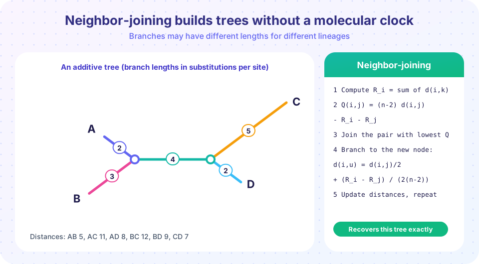
If a tree with branch lengths describes the evolution exactly, the distance between two leaves is the sum of the branch lengths on the path connecting them. Such distances are called additive. The tree in the picture has branches A:2, B:3, C:5 and D:2, joined by an internal branch of length 4. The distance from A to B is 2 + 3 = 5, from A to C is 2 + 4 + 5 = 11, from A to D is 2 + 4 + 2 = 8, from B to C is 3 + 4 + 5 = 12, from B to D is 3 + 4 + 2 = 9 and from C to D is 5 + 2 = 7.
Additive distances satisfy the four-point condition: for any four leaves, compute the three sums d(A,B) + d(C,D), d(A,C) + d(B,D) and d(A,D) + d(B,C). The two largest are equal, and the third (smallest) corresponds to the true pairing. Here the sums are 5 + 7 = 12, 11 + 9 = 20 and 8 + 12 = 20. The two largest are equal (20), and the smallest (12) identifies the grouping AB | CD. Real estimated distances are noisy and only approximately additive, but NJ still performs well.
Why UPGMA's choice is not enough
The closest pair in a matrix is not necessarily a pair of neighbors. A leaf on a very long branch is far from everything, and two leaves on very short branches look close even if they are on opposite sides of the tree. UPGMA's rule, "join the closest pair," therefore fails when rates differ. NJ fixes this by correcting each distance for how far each leaf is from all the others.
The algorithm
Let n be the number of remaining nodes, and let R_i be the sum of the distances from node i to all the others. For every pair compute
Q(i, j) = (n - 2) * d(i, j) - R_i - R_j
Join the pair with the smallest Q. The correction subtracts R_i and R_j, so a leaf far from everything is not penalized for being far. Replace i and j by a new node u. The branch lengths from i and j to u are
d(i, u) = d(i, j) / 2 + (R_i - R_j) / (2 * (n - 2))
d(j, u) = d(i, j) - d(i, u)
and the distance from u to every other node k is d(u, k) = (d(i, k) + d(j, k) - d(i, j)) / 2. Repeat until three nodes remain, then connect them in a star using (d(a,b) + d(a,c) - d(b,c)) / 2 for the branch to a, and the analogous formulas for b and c.
Worked example
Use the six distances above: AB = 5, AC = 11, AD = 8, BC = 12, BD = 9, CD = 7, with n = 4.
Net divergences: R_A = 5 + 11 + 8 = 24, R_B = 5 + 12 + 9 = 26, R_C = 11 + 12 + 7 = 30, R_D = 8 + 9 + 7 = 24.
Q values with (n - 2) = 2: Q(A,B) = 2 * 5 - 24 - 26 = -40, Q(C,D) = 2 * 7 - 30 - 24 = -40, and all other pairs give -32. The most negative is -40 for AB (tied with CD, which describes the same split). Join A and B into a node u:
d(A,u) = 5 / 2 + (24 - 26) / (2 * 2) = 2.5 - 0.5 = 2 and d(B,u) = 5 - 2 = 3. Those are exactly the true branch lengths.
New distances: d(u,C) = (11 + 12 - 5) / 2 = 9 and d(u,D) = (8 + 9 - 5) / 2 = 6. Now three nodes remain (u, C and D) with distances 9, 6 and 7. The star branch lengths are u: (9 + 6 - 7) / 2 = 4, C: (9 + 7 - 6) / 2 = 5 and D: (6 + 7 - 9) / 2 = 2. The reconstructed tree has A:2, B:3, internal 4, C:5, D:2, identical to the original.
Properties and caveats
NJ is consistent: given exactly additive distances, it returns the true tree. It runs in O(n^3) time in the simple form (faster variants such as BIONJ, FastME and RapidNJ speed it up), so it handles thousands of sequences. It makes no clock assumption, and its output is an unrooted tree; to root it you add an outgroup or use the midpoint of the longest path. In the presence of noise, NJ can produce slightly negative branch lengths, which are usually set to zero. NJ is also only as good as the distances: a poor alignment, a bad correction or saturated sequences give a poor tree, and NJ does not use character-by-character information the way parsimony or likelihood do. Many analysts use NJ for a quick first look and for large data, then confirm with maximum likelihood.
Common misconceptions
- "NJ joins the two closest sequences." It joins the pair with the smallest Q, which corrects for each leaf's distance from the rest.
- "NJ produces a rooted tree." The output is unrooted; rooting needs extra information.
- "NJ is a model-based method." It is a distance algorithm; models enter only through the distance correction you chose.
- "Negative branch lengths show a bug." They arise from noise in the distances and are usually truncated to zero.
Try it
Press Run (or Ctrl + Enter) to see the result here.
Program input · what you'd type while the program runs
Type the answers before you press Run, one per line. Each time the program reads a line (with input()), it gets the next line from this box.
Press Run (or Ctrl + Enter) to see the result here.
Program input · what you'd type while the program runs
Type the answers before you press Run, one per line. Each time the program reads a line (with input()), it gets the next line from this box.
Check your understanding
Quick check · 5 questions
of 5 answered You scored / 5 · perfect!
-
1. What does neighbor-joining do that UPGMA does not require?
NJ corrects distances by each leaf's net divergence and allows each branch its own length. -
2. Which pair does NJ join?
Q(i,j) = (n-2) d(i,j) - R_i - R_j; the minimum identifies neighbors. -
3. For the four-point condition on additive distances, which statement is true?
The smallest sum corresponds to the true pairing; the other two are equal. -
4. What is the output of NJ?
NJ gives an unrooted tree; you root it with an outgroup or midpoint. -
5. In the worked example, what is d(u,C) after joining A and B (AC = 11, BC = 12, AB = 5)?
(11 + 12 - 5) / 2 = 9.
Summary
- NJ chooses the pair with the smallest Q, corrects for net divergence and estimates branch lengths for each join.
- It returns the true tree from additive distances, with no molecular-clock assumption.
- Output is unrooted; negative branch lengths come from noise and are usually set to zero.
- It is fast and ideal for first looks and large data; confirm important results with likelihood-based methods.
Track your progress
Create a free account to tick off lessons and pick up where you left off on any device.
of Bioinformatics lessons completed