


















Lesson 31 of 49 · Transcriptomics and Expression
Differential Expression: Fold Changes, p-values and FDR
Learn how RNA-seq differential expression works: log2 fold changes, negative binomial models, Wald tests, Benjamini-Hochberg FDR control and how to read a volcano plot.
After normalization comes the central question of most RNA-seq studies: which genes changed between conditions, and can we believe it? A gene that appears twice as high in treated samples might reflect biology, or just the random wobble of counts. Differential expression analysis turns that vague feeling into an effect size (the fold change) and a measure of evidence (a p-value), and then handles the fact that you ask this question for 20,000 genes at once.
This lesson walks through the logic in the order you will meet it: fold change, the statistical model for counts, the test, the correction for multiple testing, and finally the plots you use to interpret the result. The ideas apply to DESeq2, edgeR and limma-voom, the three tools that dominate the field.
What you will learn
- How to compute and interpret a log2 fold change.
- Why RNA-seq counts need a negative binomial model, and how tools share information across genes.
- What the p-value does and does not say, and why we correct for multiple testing.
- How the Benjamini-Hochberg procedure controls the false discovery rate, step by step.
- How to read volcano and MA plots and avoid common traps.
Key terms
Log2 fold change (LFC): log2(mean expression in B / mean expression in A); 1 means doubled, -1 means halved.
p-value: the probability of seeing a difference at least this large if the gene were not really changed.
FDR (false discovery rate): the expected fraction of false positives among the genes you call significant.
Adjusted p-value (padj): the smallest FDR at which a gene would be called significant.
Dispersion: how much more variable the counts are than a Poisson distribution would be.
Effect size: the log2 fold change
The fold change tells you how big the difference is, independent of how sure you are about it. We use the base-2 logarithm because it makes up and down symmetric: a gene that doubles has LFC +1, a gene that halves has LFC -1, and a gene that is unchanged has 0. A fourfold increase is +2 and a 10-fold decrease is about -3.32.
| Ratio treated / control | log2 fold change |
|---|---|
| 8 | 3 |
| 2 | 1 |
| 1.5 | 0.585 |
| 1 | 0 |
| 0.5 | -1 |
| 0.1 | -3.32 |
Low-count genes have wildly noisy ratios (going from 1 read to 3 reads is a "threefold change" that means nothing). Modern tools therefore offer log fold change shrinkage (for example the apeglm or ashr methods in DESeq2), which pulls unreliable estimates toward zero while leaving well-measured ones alone. Use shrunken values for ranking and plotting.
The statistical model for counts
If every sample were an exact technical repeat, counts for a gene would follow a Poisson distribution, where the variance equals the mean. Real biological replicates differ from each other for reasons beyond sampling, so the variance is larger. The standard model is the negative binomial distribution, a Poisson whose rate itself varies from sample to sample:
Var(count) = mu + alpha * mu^2
where mu is the expected count and alpha is the gene's dispersion. At low counts the mu term dominates (the data behave like Poisson), and at high counts the alpha * mu^2 term dominates, so the relative noise is a constant sqrt(alpha): a gene with alpha = 0.1 has about 32% biological variation however deep you sequence. That is why sequencing more cannot replace more replicates.
With only three samples per group, estimating a separate dispersion for each gene is very unreliable. DESeq2 and edgeR use an empirical Bayes idea: fit a trend of dispersion against mean expression across all genes, then shrink each gene's own estimate toward the trend. Information is borrowed from the other 20,000 genes, which stabilizes the test and is what makes small experiments workable. Limma-voom takes a different route: it models the mean-variance relationship of log-CPM values and gives each observation a precision weight, then uses linear models.
The test
For each gene the software fits a generalized linear model with a log link in which the log of the expected count is a sum of terms from the design: an intercept, the condition, and any covariates such as batch, plus an offset for the sample's size factor. The null hypothesis is that the condition coefficient is zero. DESeq2 uses a Wald test (the coefficient divided by its standard error), or optionally a likelihood ratio test; edgeR offers a likelihood ratio test and the quasi-likelihood F-test.
Including a known nuisance factor in the design is how you handle batch: with the design ~ batch + condition, the comparison between conditions is made within each batch. In R, the DESeq2 workflow is only a few lines (shown read-only, since R is not available in this lesson's runner):
dds <- DESeqDataSetFromMatrix(countData = counts, colData = coldata,
                              design = ~ batch + condition)
dds <- DESeq(dds)
res <- results(dds, contrast = c("condition", "treated", "control"), alpha = 0.05)
head(res[order(res$padj), ])    # columns: baseMean, log2FoldChange, lfcSE, stat, pvalue, padj
The result table has one row per gene: the mean normalized count (baseMean), the LFC and its standard error, the test statistic, the raw p-value and the adjusted p-value. Genes with NA in padj were removed by outlier detection or independent filtering, which drops low-count genes that could never be significant.
Why we must correct for multiple testing
A p-value below 0.05 means: "if there were no real change, a result this extreme would happen 5% of the time". Now run 20,000 tests. Even if no gene is truly changed, about 0.05 * 20,000 = 1,000 will pass the 0.05 cut by chance. Reporting them as discoveries would be mostly false.
Two corrections are widely used:
- Bonferroni divides the threshold by the number of tests, so each test must pass
0.05 / 20,000 = 2.5e-6. It controls the chance of any false positive (the family-wise error rate) and is very conservative: you lose many real findings. - Benjamini-Hochberg (BH) controls the false discovery rate: among the genes you call significant, you expect at most a fraction
q(say 5%) to be false. It is far more powerful and is the default in nearly every RNA-seq tool.
The BH procedure, step by step
- Sort the
mp-values from smallest to largest:p(1) <= p(2) <= ... <= p(m). - Find the largest rank
ksuch thatp(k) <= (k / m) * q. - Declare genes of rank 1 to
ksignificant.
For the adjusted p-values reported in tables, compute p(i) * m / i, then enforce monotonicity by taking, from the largest rank down, the running minimum, and capping at 1.
Example with m = 6, q = 0.05:
| Rank | p | threshold (k/6) * 0.05 |
adjusted p |
|---|---|---|---|
| 1 | 0.001 | 0.0083 | 0.0060 |
| 2 | 0.008 | 0.0167 | 0.0240 |
| 3 | 0.039 | 0.0250 | 0.0504 |
| 4 | 0.041 | 0.0333 | 0.0504 |
| 5 | 0.042 | 0.0417 | 0.0504 |
| 6 | 0.600 | 0.0500 | 0.6000 |
Only ranks 1 and 2 pass. Notice that three genes with raw p of about 0.04 would have been "significant" without correction.
Reading the plots
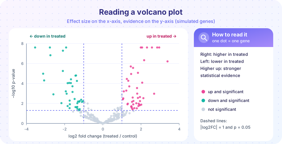
A volcano plot (the figure above) puts the effect size on the x-axis and -log10(p) on the y-axis. Genes in the upper left and upper right corners are both strongly changed and strongly supported; those low in the middle are neither. Dashed lines show the cutoffs, typically |LFC| > 1 and adjusted p below 0.05. An MA plot shows LFC against mean expression; it reveals that low-count genes scatter widely, and that a good normalization centres the cloud on zero.
A final diagnostic is the histogram of raw p-values. If most genes are null, the histogram is flat with a spike near zero for the true effects. A U-shape, a hill in the middle, or a strange spike elsewhere signals a violated assumption (for instance unmodeled batch) that no correction can fix.
Common misconceptions
"padj < 0.05 means each gene has a 5% chance of being a false positive." It means that among all the genes on your significant list, about 5% are expected to be false. Individual genes differ.
"A large fold change means a significant change." A fold change from 2 reads to 8 reads is fourfold but uninformative. Significance depends on counts and replicates as well as size.
"A gene that is not significant did not change." It means you had insufficient evidence; with more replicates you might detect it. Absence of evidence is not evidence of absence.
Try it
Run BH by hand on the six p-values from the table and compare with Bonferroni on simulated data. Then compute the fold change and Welch t-test for one gene from normalized counts. Finally, simulate a whole experiment and draw its volcano plot.
Press Run (or Ctrl + Enter) to see the result here.
Program input · what you'd type while the program runs
Type the answers before you press Run, one per line. Each time the program reads a line (with input()), it gets the next line from this box.
Press Run (or Ctrl + Enter) to see the result here.
Program input · what you'd type while the program runs
Type the answers before you press Run, one per line. Each time the program reads a line (with input()), it gets the next line from this box.
Press Run (or Ctrl + Enter) to see the result here.
Program input · what you'd type while the program runs
Type the answers before you press Run, one per line. Each time the program reads a line (with input()), it gets the next line from this box.
Check your understanding
Quick check · 5 questions
of 5 answered You scored / 5 · perfect!
-
1. A gene's mean normalized count is 50 in control and 200 in treated. What is its log2 fold change?
200 / 50 = 4 and log2(4) = 2. -
2. Why is the negative binomial distribution used for RNA-seq counts instead of the Poisson distribution?
The extra biological variation gives variance mu + alpha * mu^2, larger than the Poisson variance mu. -
3. You test 20,000 genes at p < 0.05 and none is truly changed. About how many false positives do you expect?
5% of 20,000 is 1,000. -
4. What does an FDR of 5% mean for a list of 200 significant genes?
5% of 200 is 10 expected false discoveries on average. -
5. In BH, with m = 100 tests, which threshold must the 5th smallest p-value pass at q = 0.05?
The threshold is (k / m) * q = (5 / 100) * 0.05 = 0.0025.
Summary
- The log2 fold change measures effect size (1 means doubled); shrinkage tames noisy low-count estimates.
- RNA-seq counts are modelled with a negative binomial,
Var = mu + alpha * mu^2; DESeq2 and edgeR borrow strength across genes to estimate dispersion; limma-voom weights log-CPM values. - Add known batches to the design so conditions are compared within batch.
- Thousands of tests need correction: Bonferroni is strict, Benjamini-Hochberg controls the false discovery rate and is the default.
- A volcano plot combines effect size and evidence; the p-value histogram is a good diagnostic. Significance is not importance, and non-significance is not proof of no change.
Track your progress
Create a free account to tick off lessons and pick up where you left off on any device.
of Bioinformatics lessons completed