


















Lesson 43 of 49 · Machine Learning in Biology
Chapter 8 Review: Machine Learning in Biology
Review features, evaluation metrics and pitfalls for machine learning on biological sequences, with a checklist, a worked critique of a claimed 99% classifier and a quiz.
This chapter had a single message, repeated in different forms: in biology, building a model is easy and believing it is hard. You learned to turn sequences into numbers (k-mers, one-hot grids), to fit an interpretable classifier, to measure it with confusion matrices and curves, to split data so relatives do not leak, and to train a convolution filter that finds a motif by itself.
The review gathers these into a checklist and then asks you to apply it to a realistic claim. If you can critique a result, you understand the chapter better than if you could only reproduce it.
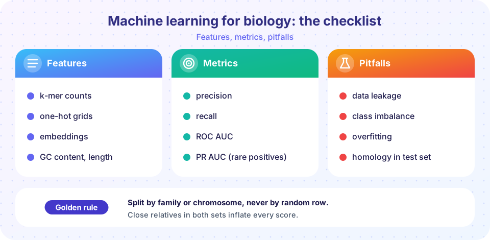
The chapter in one table
| Topic | Key facts | Lesson |
|---|---|---|
| Workflow | question and labels, features, honest split, fit, evaluate, interpret | Overview |
| Encodings | 4^k k-mer features; one-hot 4 by L grid; GC content |
Sequence features |
| Logistic regression | p = 1 / (1 + exp(-(w . x + b))); standardize with training statistics; weights are associations |
Sequence features |
| Metrics | precision TP / (TP + FP), recall TP / (TP + FN), ROC AUC, average precision |
Evaluating classifiers |
| Splitting | train/validation/test; group by family, cluster or chromosome | Evaluating classifiers |
| Deep learning | convolution = learned motif scanner; max pooling; embeddings; transfer learning | Deep learning |
Ideas that connect the lessons
The representation is a hypothesis. Choosing k-mers says "composition matters, order does not"; choosing one-hot with a convolution says "local patterns matter wherever they occur". If the hypothesis does not match the biology, no algorithm will rescue it. The same data, encoded differently, gave very different accuracy in the experiment.
The evaluation is also a hypothesis. A random split says "my future data are like a random sample of this dataset". In biology, future data are usually new families, species or individuals, so a family-aware split is the honest simulation of that future. The leakage experiment, with labels that were pure noise, showed that a random split can reward memorization.
Simple baselines protect you. A threshold on GC content, a logistic regression on k-mers and a shuffled-label control cost minutes and tell you what a complicated model has to beat. When the baseline is already near the ceiling, the deep model is solving a problem that did not need it.
Interpretability is a check, not a decoration. Reading a regression's weights or a filter's motif tells you whether the model found the biology or a shortcut. An uninterpretable high score should make you more suspicious, not less.
A reproducible checklist
- Question and labels: Where did each label come from, how noisy is it, and who is missing from the data?
- Class balance: What fraction is positive? State the baseline precision and what a trivial classifier scores.
- Features: Do they match the pattern you expect (local motif, composition, position-specific)? Are the scalings computed on training data only?
- Split: Are relatives, duplicates and the same patient kept on one side? Is the test set untouched until the end?
- Metrics: Report precision, recall, ROC AUC and average precision with confidence intervals, plus a simple baseline and a shuffled-label control.
- Interpretation: What did the model learn, and does it make biological sense? Is there an independent validation set from a different source?
Worked example: "99% accurate"
A preprint claims a deep network that classifies variants as pathogenic or benign with 99% accuracy. Apply the checklist.
Balance. In many databases benign variants outnumber pathogenic ones by a large factor, or the reverse in a curated set. If 98% of the test variants are benign, 99% accuracy is barely above the trivial baseline. Ask for precision, recall and average precision on the pathogenic class.
Labels. The authors took labels from a public clinical database. Those labels were partly assigned by computational predictors, so training a predictor on them can partly learn the older predictors' rules (circularity).
Split. Variants in the same gene tend to share a label, because a gene is either dosage-sensitive or not. If the split is random across variants, the model can score highly by learning "this gene is a disease gene" instead of judging individual variants. A split that holds out whole genes is the realistic test.
Evidence of leakage. Does a gene-level baseline that ignores the variant (just the gene's overall pathogenic fraction) get close to 99%? If yes, the network may have learned little beyond that.
After these questions, the claim might shrink to something like 80% on a gene-held-out set, which is still useful, but it is a different statement from "99% accurate". Knowing how to reduce a headline to the honest number is the practical payoff of the chapter.
Connecting the chapter to the rest of the course
Machine learning is not a separate island. The Phred idea from the genomics chapter returns here whenever a model outputs a probability: a well-calibrated model that says 0.9 should be right about nine times in ten, which is the same logic as a base called at Q10. The multiple-testing problem from the RNA-seq chapter returns when you try many models, many hyperparameters or many feature sets on one test set, because each attempt is another test and the best result is flattered by selection. The distance-based thinking of the structure chapter returns in embeddings, where similar proteins end up near each other in a vector space and "similar" is measured with distances.
The projects in the next chapter use these links on purpose. The variant caller applies Bayes' rule and priors, which is the same reasoning a probabilistic classifier uses, and the RNA-seq project evaluates a pipeline against known truth with precision, recall and a power curve, which is the evaluation discipline of this chapter applied to a statistical test.
Reading the literature with this checklist
The questions above also work as a reading strategy. When a paper reports a new predictor, look first for the table that describes the dataset: how many positives and negatives, where the labels came from, and how the split was made. Then look for the baselines: if the only comparison is with older, weaker methods and not with a simple model, the benefit is unclear. Look for an external test set from a different source or time, because performance on data collected another way is the strongest evidence that the model learned something general. Finally, look at what the authors did when the model was wrong: papers that show failure cases and discuss them honestly are usually more trustworthy than papers that show only successes.
You do not have to distrust every result. The point is to know which questions to ask, so that a good result can earn your confidence and a weak one cannot borrow it.
Try it
The first example turns a few facts about a dataset into a list of warnings, a miniature checklist. The second is an interactive threshold explorer: move the score threshold and class prevalence sliders to see how precision and recall change.
Press Run (or Ctrl + Enter) to see the result here.
Program input · what you'd type while the program runs
Type the answers before you press Run, one per line. Each time the program reads a line (with input()), it gets the next line from this box.
Check your understanding
Quick check · 9 questions
of 9 answered You scored / 9 · perfect!
-
1. How many 5-mer features are possible for DNA?
4^5 = 1,024. -
2. A test set has 2% positives. A model that always predicts negative has accuracy of:
It is right for every negative example, 98% of the data. -
3. Which metric combination is most informative when positives are rare?
They focus on the positive class, unlike accuracy and ROC-based numbers that the large negative class can inflate. -
4. What is the best way to split a dataset of protein sequences for evaluation?
Cluster-aware splitting stops close relatives from appearing on both sides. -
5. A model trained on shuffled labels scores AUC 0.8. What does it indicate?
Shuffling destroys real signal, so a high score means information is leaking. -
6. A one-filter convolution with global max pooling is best described as:
The filter slides along the sequence and max pooling keeps the strongest match anywhere. -
7. Why standardize features with training-set statistics only?
Computing means and deviations on all data lets test information influence preprocessing. -
8. What does lowering the decision threshold usually do?
More examples are called positive, so more true positives are found but more false alarms appear. -
9. A deep network on 300 labeled sequences barely beats a k-mer logistic regression. The sensible conclusion is:
With little data, simple, interpretable baselines are often as good and easier to trust.
Summary
- Pick features that match the biology: k-mer counts for composition, one-hot with convolutions for local patterns at any position.
- Evaluate with precision, recall, ROC AUC and average precision, always next to a baseline and the class balance.
- Split by family, cluster or chromosome; test shuffled labels to detect leaks.
- Interpret what the model learned, and validate on independent data before believing a headline number.
Track your progress
Create a free account to tick off lessons and pick up where you left off on any device.
of Bioinformatics lessons completed