


















Lesson 14 of 49 · Sequence Alignment
Local alignment: Smith-Waterman
Learn local alignment with the Smith-Waterman algorithm: the zero floor, finding the best matching region, traceback, why the expected score must be negative, and Python code.
Needleman-Wunsch aligns two sequences from end to end. That is the wrong question for many real problems. A 2,000-residue enzyme and a 150-residue protein may share only a 90-residue domain; a bacterial genome and a gene may overlap in a short stretch. Forcing an end-to-end alignment drags the unrelated flanks into the score and hides the interesting part. In 1981 Temple Smith and Michael Waterman showed that one small change to the recurrence turns the global method into a local one that finds the best-matching region of any two sequences.
What you will learn
- The single change that turns Needleman-Wunsch into Smith-Waterman.
- Where a local alignment starts and ends, and how to trace it back.
- Why random local scores stay low only if the expected pair score is negative.
- When to choose local, global or semi-global alignment.
Key terms
- Local alignment: the best-scoring alignment of any pair of substrings, one from each sequence.
- Zero floor: the rule that a cell's score is never allowed to drop below 0, which means "start over here".
- Semi-global (glocal) alignment: one sequence is aligned end to end against part of the other, as when fitting a read to a reference.
- Expected score: the average score of a random residue pair under the scoring scheme.
- Extreme-value distribution: the distribution of the best score among many random alignments.
One change: a floor of zero
The local recurrence is almost identical to the global one:
H(i, j) = max(
    0,                              # start a new local alignment here
    H(i-1, j-1) + s(a_i, b_j),
    H(i-1, j)   + gap,
    H(i,   j-1) + gap
)
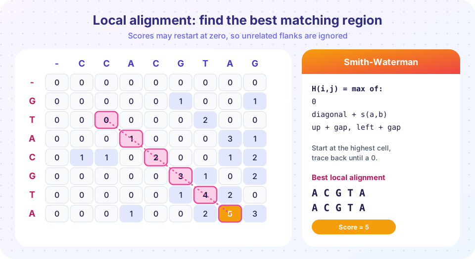
The first option, 0, lets any cell restart the alignment. If the best way to align two prefixes ends in a negative-scoring stretch, the algorithm simply discards the stretch and starts again. Consequently the first row and the first column are all zeros (no penalty for leaving the start of either sequence unaligned) and the matrix contains no negative values.
Two further changes follow. The end of the best local alignment is not the bottom-right corner but the cell with the highest value anywhere in the matrix. And the traceback starts from that cell and stops as soon as it reaches a cell with value 0, since the alignment began just after that cell.
Worked example
Let a = GTACGTA (down the side) and b = CCACGTAG (across). They share the stretch ACGTA. With +1 for a match, -1 for a mismatch and -2 for a gap, the matrix fills as follows. Cell (3, 3), where A meets A, gets H(2,2) + 1. That diagonal neighbor is 0, so the cell is 1. The next diagonal cell (4, 4), C against C, becomes 2, then (5, 5) G against G is 3, (6, 6) T against T is 4, and (7, 7) A against A is 5. The highest cell in the matrix is 5. Tracing back diagonally leads through 4, 3, 2, 1 down to the zero at (2, 2) and the alignment is
A C G T A
A C G T A
with score 5. The other letters (GT at the start of a, and CC and G in b) are simply left out. A global alignment of the same two sequences would have to pay for all of them.
Why the expected score must be negative
There is a subtle condition. Suppose the scoring scheme gave a positive average score to a random pair of residues. Then longer and longer alignments would score higher on average even for unrelated sequences, and the best local alignment would stretch across everything, meaning nothing. For local alignment to mean something, the expected score of a random pair must be negative, while at least some pairs score positive. With +1 for a match and -1 for a mismatch in random DNA, the expected pair score is 0.25(+1) + 0.75(-1) = -0.5, which is fine. Karlin and Altschul (1990) showed that when this condition holds, the best local score between random sequences follows an extreme-value (Gumbel) distribution, and the score grows only with the logarithm of the sequence lengths. This theory is the foundation of the E-values you will meet in the BLAST lesson.
Choosing the right flavor
| Situation | Method |
|---|---|
| Two versions of one gene, expected to match end to end | Global (Needleman-Wunsch) |
| A shared domain or motif inside longer sequences | Local (Smith-Waterman) |
| A short read inside a long reference | Semi-global: read fully aligned, reference ends free |
| A query against a huge database | Local, but by heuristic (BLAST) |
Smith-Waterman gives the mathematically optimal local alignment, but its cost is O(mn), too slow for searching a large database one sequence at a time. Optimized implementations exploit processor vector instructions and run many times faster, and BLAST and its relatives gain their speed by examining only promising regions, as you will see next.
Local alignment in practice
Local alignment is the workhorse for finding domains, motifs and repeats. Consider a protein kinase domain of about 250 residues embedded in two very different proteins of 800 and 1,200 residues. A global alignment of the two would be dominated by unrelated flanks and would score poorly. A local alignment ignores the flanks and reports the domain, with a score that reflects how conserved it is. Many tools you will meet rely on local alignment: BLAST, Pfam and HMMER searches, and short-read mappers that use local alignment to allow reads with adapter or poor-quality ends to be soft-clipped (the unaligned ends are retained in the file but not scored).
Local alignment also works with the affine gap penalties from the previous lesson. The recurrence then needs three matrices, as in the global case, and each keeps the zero floor. Finally, think about statistics. Because the algorithm reports the best score out of all possible start and end points, a high score is easier to reach by chance for longer sequences, which is why the significance of a local alignment must be judged with E-values and not with the raw score alone, a topic the BLAST lesson picks up next.
Common misconceptions
- "Local alignments are always shorter and therefore less reliable." Length matters less than score and its statistical significance.
- "The traceback ends at the top-left corner." It ends at a zero cell, which can be anywhere.
- "I can use any scoring scheme with Smith-Waterman." The expected random score must be negative, or the output is meaningless.
- "A local alignment finds all shared regions." The basic algorithm reports only the best one. Finding several needs repeated runs or extensions of the algorithm.
Try it
Press Run (or Ctrl + Enter) to see the result here.
Program input · what you'd type while the program runs
Type the answers before you press Run, one per line. Each time the program reads a line (with input()), it gets the next line from this box.
Press Run (or Ctrl + Enter) to see the result here.
Program input · what you'd type while the program runs
Type the answers before you press Run, one per line. Each time the program reads a line (with input()), it gets the next line from this box.
Check your understanding
Quick check · 5 questions
of 5 answered You scored / 5 · perfect!
-
1. What is the key change from Needleman-Wunsch to Smith-Waterman?
Adding 0 as a fourth option in the recurrence lets the alignment restart anywhere. -
2. Where does the traceback of a local alignment start?
The best local alignment ends at the maximum cell and is traced back until a zero. -
3. Why must the expected score of a random residue pair be negative?
A positive expected score makes scores grow with length even for unrelated sequences. -
4. A 120-base read must be aligned in full inside a 5,000-base reference. Which method fits best?
The whole read is aligned while the reference ends are free: semi-global alignment. -
5. What distribution describes the maximum local score between random sequences?
Karlin and Altschul showed that maxima of local scores follow an extreme-value distribution.
Summary
- Smith-Waterman adds a floor of 0 to the recurrence, so alignments can start anywhere.
- The best local alignment ends at the matrix maximum and is traced back to a zero.
- Local alignment needs a negative expected score for random pairs; its random maxima follow an extreme-value distribution.
- Use local alignment for shared regions, global for full-length relatives and semi-global for reads in references.
Track your progress
Create a free account to tick off lessons and pick up where you left off on any device.
of Bioinformatics lessons completed