


















Lesson 30 of 49 · Transcriptomics and Expression
RNA-seq Counts and Normalization: CPM, TPM and Size Factors
Learn why raw RNA-seq counts mislead and how CPM, TPM, TMM and the median-of-ratios method correct for sequencing depth, gene length and composition bias.
A count matrix looks like the answer: a table of numbers, one per gene per sample. It is tempting to compare them directly. But if sample 1 was sequenced to 20 million reads and sample 2 to 40 million, every gene in sample 2 will have about twice as many reads, and nothing about the biology has changed. Likewise, a long gene collects more reads than a short gene expressed at the same level.
Normalization is the set of corrections that make numbers comparable. It is also the part of RNA-seq analysis that is easiest to do wrongly, because there are several methods, each correct for a particular question. In this lesson you will learn what each one fixes, which one to use for which job, and how to compute them yourself.
What you will learn
- The three distortions in raw counts: sequencing depth, gene length and composition.
- How to compute CPM, RPKM/FPKM and TPM, and why TPM is preferred for within-sample comparison.
- How the median-of-ratios and TMM methods find size factors for between-sample comparison.
- When to use raw counts, normalized counts or log-transformed values.
Key terms
Library size: the total number of reads (or assigned reads) in a sample.
CPM: counts per million, count / library size * 10^6.
TPM: transcripts per million, a length-aware measure that always sums to one million per sample.
Size factor: a per-sample number that scales counts so samples are comparable.
Composition bias: distortion caused when a few extremely abundant genes take up a large share of the reads.
Three distortions in raw counts
Depth. Sequencing 40 million reads instead of 20 million doubles counts everywhere. This is the obvious one, and dividing by library size fixes it.
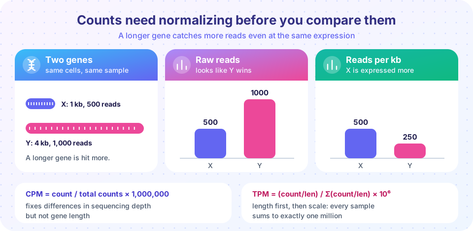
Gene length. A transcript fragmented into pieces gives reads in proportion to its length. Two genes with the same number of mRNA molecules but lengths of 1 kb and 4 kb will produce reads in a 1 to 4 ratio. The figure above shows this: gene Y has twice the reads of gene X, yet per kilobase it has half as many. If you want to ask "which of these two genes has more transcripts in this sample?", you must divide by length.
Composition. Suppose in condition B one gene explodes and consumes 30% of all reads. Every other gene's share falls, so their counts drop in proportion even though nothing happened to them. A method that only divides by total reads will then report a spurious decrease in thousands of genes. This is a subtle effect, and it is the reason between-sample normalization is more careful than "divide by the total".
Which distortion matters depends on the question:
| Question | Compare | Fix needed |
|---|---|---|
| Is gene A higher in treated than control? | the same gene across samples | depth and composition (length cancels out) |
| Is gene A more expressed than gene B in one sample? | different genes in one sample | length (and depth) |
| Do these samples cluster together? | all genes across samples | depth and composition, plus a variance-stabilizing transform |
Within-sample measures: CPM, RPKM and TPM
CPM scales by library size only:
CPM = count / total counts * 1,000,000
It is good for filtering and plotting, but ignores length.
RPKM (reads per kilobase per million) and its paired-end version FPKM were the earlier standard. They divide by library size in millions, then by gene length in kilobases:
RPKM = count / (length in kb * total counts in millions)
TPM (transcripts per million) reverses the order: divide each count by the gene length first, then scale so the sample adds up to one million:
TPM = (count / length) / sum over all genes of (count / length) * 1,000,000
Reversing the order has a useful consequence. In every sample the TPM values sum to exactly one million, so a TPM of 50 means "50 out of every million transcripts in this sample", which makes values from different samples more directly comparable as proportions. RPKM sums vary from sample to sample, which makes the same value mean different things in different samples. That is why TPM is generally preferred when you need a within-sample abundance measure.
TPM is still relative. It tells you the share of the transcript pool, not the absolute number of molecules per cell, and it still suffers from composition effects between samples.
Between-sample normalization: size factors
For differential expression, statistical packages work on raw counts and estimate a size factor per sample that enters the model as an offset, accounting for depth and composition together.
The median-of-ratios method (DESeq2)
- For each gene, compute the geometric mean of its counts across all samples (only genes with nonzero counts in every sample can be used).
- For each sample and gene, divide the count by that geometric mean: this is the gene's "ratio" in that sample.
- The sample's size factor is the median of its ratios across genes.
- Normalized counts are
count / size factor.
The median is the key. Most genes do not change between conditions, so the typical ratio reflects the sample's sequencing effort; a few strongly changed genes are outliers that the median ignores. In the exercise below you will see total-count normalization get fooled by one exploding gene while the median-of-ratios stays correct.
TMM (edgeR)
The trimmed mean of M-values takes a reference sample and, for each other sample, computes the log fold change (M) and the average abundance (A) of every gene. It trims away the most extreme M and A values (30% of M and 5% of A by default) and takes a weighted mean of the rest, which becomes a scaling factor combined with library size. The two methods rest on the same assumption, that most genes are not differentially expressed, and they usually agree closely.
Transformations for plotting and clustering
Counts have a variance that grows with the mean, so highly expressed genes dominate distance calculations and plots. For visualization, PCA and clustering you transform the normalized counts:
- log2(CPM + 1) (or
log2(normalized count + 1)): easy and often adequate; the pseudo-count of 1 avoidslog(0). - VST (variance stabilizing transformation) or rlog from DESeq2: build in the mean-variance trend and behave better for low counts.
Never run the statistical test itself on log-transformed or TPM values with a count-based tool: DESeq2 and edgeR model the raw counts with a negative binomial distribution and expect integers. Feeding them TPM discards the information that tells them how much sampling noise each gene has.
Filtering low-count genes
Genes with almost no reads carry no signal, add noise, and increase the multiple-testing burden. A typical rule keeps genes with a CPM above a threshold (corresponding to roughly 5 to 10 reads) in at least as many samples as the smallest group. DESeq2 also performs independent filtering internally.
Common misconceptions
"TPM is the absolute number of transcripts." It is a proportion of the transcript pool in a sample, so it cannot say that one sample has more total RNA than another.
"Use TPM or FPKM values as the input to DESeq2 or edgeR." Both want raw counts; they handle depth through their own size factors.
"Normalization removes biological differences." It removes technical differences in depth and composition. A well-normalized dataset should still show the real changes, and a normalization that erases them (for instance, when most genes truly change) is a warning that its assumption failed.
Try it
Compute CPM, RPKM and TPM for a handful of genes in two samples. Next, implement the median-of-ratios method and compare it with total-count scaling when one gene explodes. Finally, simulate samples with different depths and see the boxplots line up after normalization.
Press Run (or Ctrl + Enter) to see the result here.
Program input · what you'd type while the program runs
Type the answers before you press Run, one per line. Each time the program reads a line (with input()), it gets the next line from this box.
Press Run (or Ctrl + Enter) to see the result here.
Program input · what you'd type while the program runs
Type the answers before you press Run, one per line. Each time the program reads a line (with input()), it gets the next line from this box.
Press Run (or Ctrl + Enter) to see the result here.
Program input · what you'd type while the program runs
Type the answers before you press Run, one per line. Each time the program reads a line (with input()), it gets the next line from this box.
Check your understanding
Quick check · 5 questions
of 5 answered You scored / 5 · perfect!
-
1. Gene X (1 kb) has 500 reads and gene Y (4 kb) has 1,000 reads in the same sample. Which statement is true?
Reads per kilobase corrects for length: 500 / 1 = 500 versus 1,000 / 4 = 250. -
2. Which measure always sums to one million in every sample?
TPM divides by length first and then rescales each sample to sum to 1,000,000. -
3. What kind of input do DESeq2 and edgeR expect for the statistical test?
They model raw counts with a negative binomial distribution and use size factors internally. -
4. Why does the median-of-ratios method resist a few strongly changed genes?
Most genes are assumed not to change, so the median ratio reflects depth and is not moved by a few outliers. -
5. For clustering and PCA of samples you should use:
Count variance grows with the mean, so a transform keeps highly expressed genes from dominating distances.
Summary
- Raw counts reflect depth, gene length and composition as well as biology.
- CPM fixes depth; RPKM/FPKM add length; TPM divides by length first and always sums to one million, which suits within-sample comparison.
- For differential expression, give DESeq2 or edgeR raw counts; they compute size factors (median-of-ratios or TMM) that handle depth and composition.
- Use log2(x + 1) or VST/rlog values for plots, PCA and clustering, and filter genes with almost no counts.
- All methods assume most genes do not change; check that assumption when a result looks strange.
Next: Differential Expression
Track your progress
Create a free account to tick off lessons and pick up where you left off on any device.
of Bioinformatics lessons completed