


















Lesson 42 of 49 · Machine Learning in Biology
Deep Learning for Sequences: Convolution Filters and Embeddings
See how convolutional filters act as learned motif scanners, train one from scratch in NumPy, and meet language-model embeddings, interpretation methods and the limits of deep learning.
In the last two lessons you chose how to turn sequences into numbers by hand: GC content, k-mer counts, one-hot grids. Deep learning flips the arrangement. You give the model the raw one-hot sequence and let it learn its own features. The key trick for sequences is the convolution: a small pattern detector, the filter, that slides along the whole sequence and reports where it matches.
If that sounds familiar, it should. A position weight matrix, the classical biological model of a motif, is a filter. A convolutional neural network is a stack of learned filters, and the weights in the first layer often turn out to be recognizable motifs. This lesson builds one filter from scratch so you can watch it discover a motif, then surveys what modern deep models do with DNA and proteins.
What you will learn
- How a convolution over a one-hot sequence works and why it detects motifs at any position.
- How a filter is trained by gradient descent, step by step.
- What pooling, ReLU and dense layers add in a full network.
- What embeddings and sequence language models are, and how they are used.
- How to interpret what a network learned, and its main limits.
Key terms
Convolution (filter): a small weight matrix applied at every position of the input, producing a score per position.
Max pooling: keeping only the largest score, which makes the result independent of position.
Embedding: a learned vector of numbers that represents a token, such as an amino acid or a whole protein.
Backpropagation: computing the gradient of the loss with respect to every weight by the chain rule.
Language model: a model trained to predict masked or next tokens, learning the statistics of sequences.
The convolution idea
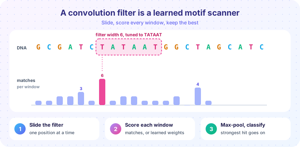
Take a one-hot encoded DNA sequence as a matrix with L rows (positions) and 4 columns (A, C, G, T). A filter of width 6 is a 6 by 4 matrix of weights. To apply it at position i, multiply the filter elementwise with rows i to i+5 of the sequence and add up the results. If the weights are +1 for the base TATAAT expects at each position and 0 elsewhere, the sum counts how many of the six positions match the motif: 6 for a perfect hit. Sliding the filter along the sequence gives a score profile with L - 6 + 1 values, exactly the bar chart in the figure above.
Two properties make this powerful:
- Weight sharing. One small set of weights is reused at every position, so a motif is detected wherever it occurs. That solves the floating-motif problem that defeated the flattened one-hot model in the earlier lesson.
- Few parameters. A filter has 24 weights regardless of the sequence length, so models can be trained on moderate amounts of data.
After the convolution, a pooling step summarizes the profile. Global max pooling keeps only the strongest score, answering the question "does the motif appear anywhere?" Local pooling (taking the maximum in small windows) keeps rough positional information. Then a dense (fully connected) layer combines the pooled values from all the filters into a prediction, often followed by a sigmoid to give a probability. Real networks use dozens to hundreds of filters, a ReLU nonlinearity (max(0, x)) after the convolution, and several layers, so that early filters detect short motifs and later layers detect combinations and spacing of motifs. Because DNA has two strands, models are often trained with the reverse complement of each sequence as extra data, or built to treat both strands the same way.
How a filter learns
Training starts with small random weights. For each example the network computes a score, turns it into a probability, and compares it with the label using the cross-entropy loss. Backpropagation applies the chain rule to find how each weight should change to reduce the loss. For a model with one filter, global max pooling and a logistic output the gradient is simple:
- For each sequence, the max-pooled score
mcomes from one best-matching window. - The gradient with respect to the filter weights is the sum over sequences of
(p - y) * a * window, wherewindowis the one-hot content of that sequence's best window. - Move the weights a small step against the gradient.
In words: for a positive sequence whose output is too low, the filter is nudged toward the content of its best window, so it learns to match what positive sequences contain; for a negative sequence with a high score, the filter is nudged away from its best window. After many steps, the filter drifts toward the pattern that separates the classes. Frameworks such as PyTorch and TensorFlow compute these gradients automatically on a GPU, but there is no magic beyond the chain rule. The example below does it by hand in NumPy.
For reference, a typical Keras definition of such a network looks like this (read-only; training it needs a library that this lesson's runner does not load):
from tensorflow import keras

model = keras.Sequential([
    keras.layers.Input(shape=(200, 4)),                      # 200 bases, one-hot
    keras.layers.Conv1D(64, 12, activation="relu"),          # 64 filters of width 12
    keras.layers.GlobalMaxPooling1D(),
    keras.layers.Dense(32, activation="relu"),
    keras.layers.Dense(1, activation="sigmoid"),             # probability of class 1
])
model.compile(optimizer="adam", loss="binary_crossentropy", metrics=["AUC"])
From one-hot to learned representations
Beyond hand-made inputs, large pretrained models learn representations from the statistics of sequences themselves.
Embeddings. An embedding is a learned vector, typically tens to thousands of numbers, standing for a token. Instead of the sparse one-hot vector for an amino acid, a model can use a dense vector learned so that similar residues sit close together.
Protein language models. Models such as ESM-2 (from Meta) and ProtTrans are trained on hundreds of millions of protein sequences to predict masked residues, the way text language models predict masked words. To do this well they must learn which residues are conserved, which co-vary and what folds look like. The resulting per-residue and per-protein embeddings carry information about structure and function, and are used as features for downstream tasks such as predicting stability, localization or the effect of a mutation, often with only a small labeled dataset. This is transfer learning: learn broadly from unlabeled data, then adapt cheaply to a specific task. ESMFold even predicts structure from such a model alone.
DNA models. Several architectures take DNA as input. DeepBind (2015), DeepSEA (2015) and Basset (2016) used convolutional networks to predict protein binding and chromatin features from sequence. Enformer (2021) used attention (a transformer) over about 200 kilobases to predict gene expression and chromatin tracks. DNA language models such as DNABERT and the Nucleotide Transformer learn from genomes without labels. AlphaMissense (2023) predicts the pathogenicity of missense variants by combining structure-aware models with evolutionary information. These systems are active research tools; their predictions are hypotheses, not diagnoses.
Looking inside the network
Neural networks are often called black boxes, but you can probe them:
- Filter visualization. Convert first-layer filters into position weight matrices and compare them with databases of known motifs.
- In silico mutagenesis. Change each base in a sequence, one at a time, and record how the prediction moves. Large drops mark important positions.
- Attribution methods such as saliency maps, integrated gradients and DeepLIFT assign a contribution to each input base.
These tools show what the model uses, which is not always what the biology uses. If a model leans on a repetitive element because it differs between your positives and negatives, interpretation will show you the shortcut.
Limits and good practice
- Data hunger. Networks with millions of parameters need much more data than logistic regression. With a few hundred examples, a simple model on k-mers is often just as good.
- Shortcuts and confounders. Networks readily exploit differences in GC content, repeats or source lab. Match controls carefully.
- Leakage. The evaluation lessons apply with full force: split by family, chromosome or species.
- Calibration. Outputs are not guaranteed to be true probabilities; check calibration if you rely on them.
- Reproducibility. Random initialization changes results; report the spread over several runs.
Common misconceptions
"Deep learning discovers biology automatically." It finds patterns predictive in your dataset, including artifacts. Interpretation and independent validation are what turn patterns into biology.
"Bigger networks are always better." On small datasets, large models overfit; start with a baseline and add capacity only when it pays off on a leak-free test set.
"An embedding is a fact about the protein." It is a learned summary of statistics in the training data, and it can be wrong for unusual or poorly represented proteins.
Try it
First, a hand-set filter finds TATAAT in a sequence. Second, a one-filter network is trained from scratch in NumPy and its learned weights are plotted; look at whether they spell the motif. Third, scan your own sequence in the browser.
Press Run (or Ctrl + Enter) to see the result here.
Program input · what you'd type while the program runs
Type the answers before you press Run, one per line. Each time the program reads a line (with input()), it gets the next line from this box.
Press Run (or Ctrl + Enter) to see the result here.
Program input · what you'd type while the program runs
Type the answers before you press Run, one per line. Each time the program reads a line (with input()), it gets the next line from this box.
Reading the trained filter
When you run the second example, the filter recovers the planted motif without ever being told what it is, but it may not line up perfectly. In a typical run the consensus reads TTATAA, which is TATAAT shifted by one position: the filter and the motif overlap almost completely, and because the filter is exactly as wide as the motif there is little penalty for sliding by one base and matching TATAA plus a neighboring T. Real networks use filters wider than the motifs they seek, so the motif sits inside the filter with near-zero weights on either side, which makes the alignment less ambiguous. The test accuracy (a little under 0.8 in our run) is also lower than a perfect score because the motif is fuzzy: with 10% mutation per base, many positive sequences contain a damaged copy that is hard to tell from a chance match. Try changing the mutation probability from 0.1 to 0.0 and see how the accuracy and the filter change.
Check your understanding
Quick check · 5 questions
of 5 answered You scored / 5 · perfect!
-
1. Why can a convolution filter find a motif wherever it occurs in a sequence?
Weight sharing makes the detector translation invariant. -
2. What does global max pooling keep from the score profile?
It answers whether the pattern occurs anywhere, regardless of position. -
3. How many weights does a filter of width 12 over a one-hot DNA sequence have?
The filter is 12 positions by 4 bases = 48 weights, independent of sequence length. -
4. In-silico mutagenesis means:
It is a computational probe of which positions the model's prediction depends on. -
5. A protein language model is first trained on millions of unlabeled sequences, then adapted to a small labeled task. This is called:
Pretraining on unlabeled data and adapting to a specific task is transfer learning.
Summary
- A convolution filter is a learned position weight matrix applied at every position; max pooling answers "is it anywhere?".
- Weight sharing gives translation invariance and few parameters, fixing the floating-motif problem of flattened one-hot models.
- Filters are trained by gradient descent: nudge each filter toward the windows it should match and away from those it should not.
- Embeddings and protein or DNA language models learn representations from unlabeled sequence and support transfer learning.
- Interpret with filter motifs, in silico mutagenesis and attribution; watch for data hunger, shortcuts and leakage.
Track your progress
Create a free account to tick off lessons and pick up where you left off on any device.
of Bioinformatics lessons completed