


















Lesson 44 of 49 · Projects and Practice
Project: Build a Toy Variant Caller
Build a miniature genomics pipeline in Python: simulate a diploid sample with sequencing errors, count bases in a pileup, call genotypes with a binomial model and measure accuracy.
Reading about variant calling is one thing; building a caller teaches you where the difficulty really lies. In this project you will create a miniature genomics pipeline entirely in Python. You will simulate a genome and a diploid sample with known variants, generate noisy reads from it, build a pileup (a table of base counts at each position), call genotypes with the binomial model from the variant-calling lesson, and then do something real pipelines rarely get to do: compare your calls with the ground truth.
Because you know the truth, you can ask the questions that matter. How many variants did the caller find? How many did it invent? How does performance change as sequencing depth falls? The answers show why a 30x coverage target exists and why low-coverage projects need caution.
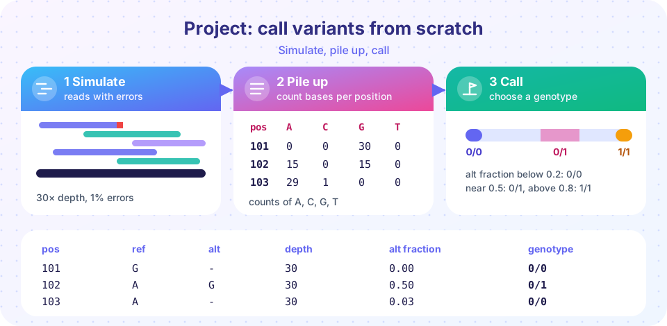
What you will build
By the end you will have a script that:
- Simulates a 400-base reference and a diploid sample with twelve true variants, a third of them homozygous.
- Generates reads from both haplotypes with a 1% per-base error rate and tallies a pileup.
- Calls each position's genotype with Bayes' rule and reports QUAL.
- Scores the calls: true positives, false positives, false negatives, and genotype accuracy.
- Sweeps sequencing depth to measure sensitivity and precision.
Key terms
Pileup: for every reference position, the count of each base seen in reads that cover it.
Ground truth: the known variants in a simulation, used to grade the caller.
Sensitivity (recall): the fraction of true variants that were found.
Precision: the fraction of called variants that are true.
Genotype accuracy: among true variants found, the fraction with the right genotype.
Step 1: simulate the sample and the reads
The reference is random DNA. The diploid sample has two haplotypes, each a copy of the reference. At twelve randomly chosen sites we introduce an alternate base: one third as homozygous alternate (both haplotypes carry it, genotype 1/1), the rest as heterozygous (only haplotype 1 carries it, genotype 0/1).
To make reads, repeat: choose a haplotype at random, choose a start position, copy 40 bases, then flip each base to a random different base with probability 0.01 (the sequencing error). Add the base counts of the read to a table counts[position, base]; that table is the pileup. The number of reads is depth * L / read_length, which is just the definition of mean depth turned around.
Run the first example to see the simulation and the pileup at the true variant sites.
Press Run (or Ctrl + Enter) to see the result here.
Program input · what you'd type while the program runs
Type the answers before you press Run, one per line. Each time the program reads a line (with input()), it gets the next line from this box.
Step 2: call genotypes with Bayes' rule
At each position take the reference base and the most common non-reference base (the candidate alternate). Let n be the depth and k the candidate's count. Under the three genotypes k follows a binomial distribution with probability e (error rate), 0.5 and 1 - e for 0/0, 0/1 and 1/1. Multiply each likelihood by a prior (most positions are reference, so use 0.998, 0.001, 0.001), normalize, and report the genotype with the highest posterior. Define QUAL = -10 * log10(P(0/0 | data)): the Phred-scaled confidence that the site is variant. Call a variant when the best genotype is not 0/0 and QUAL >= 20, which means a posterior of 99% or more that the site differs from the reference.
Then grade the calls. A call is a true positive if the position is in the truth set. It is a genotype match if the genotype agrees. Calls at other positions are false positives, and truth sites without a call are false negatives.
Press Run (or Ctrl + Enter) to see the result here.
Program input · what you'd type while the program runs
Type the answers before you press Run, one per line. Each time the program reads a line (with input()), it gets the next line from this box.
Step 3: how does depth change the answer?
A caller's performance depends on the evidence it has. At 2x depth a heterozygous site might have 2 reads, and both could carry the reference base by chance, so the site goes unseen. At 40x there is rarely any doubt. The next script varies the depth, repeats the experiment with several random seeds, and plots sensitivity and precision.
Press Run (or Ctrl + Enter) to see the result here.
Program input · what you'd type while the program runs
Type the answers before you press Run, one per line. Each time the program reads a line (with input()), it gets the next line from this box.
Reading the results
With 30x depth your caller should find essentially all twelve variants with correct genotypes and no false positives, because the evidence is overwhelming: heterozygous sites show alternate fractions near 0.5 on dozens of reads, and error-only sites show a few alternate reads at most. Dropping to 4x or 6x depth costs sensitivity, mostly through heterozygous sites whose alternate reads are too few to pass the quality threshold, and homozygous sites are called more reliably than heterozygous ones because their signal is stronger. Precision stays high across depths in this clean simulation because errors are uniform and independent. Real data are less kind: errors cluster in particular sequence contexts, mapping mistakes put reads in the wrong place, and repeats attract false alternate reads, which is why real pipelines add filters on strand bias, mapping quality and depth.
Design decisions, and what they teach
Every line of the simulator and the caller embodies a choice, and each choice mirrors a decision in a real pipeline.
Why the prior is so strong. Setting the reference prior to 0.998 means the caller needs about a thousand-to-one evidence to overturn it. In human data variants occur at roughly one position in a thousand, so the prior is realistic, and it explains why two alternate reads at a depth of six are not enough. Try an unrealistic prior of one third for each genotype and you will see the caller invent many false positives at low depth, a good demonstration of how a model's assumptions control its behavior when evidence is thin.
Why QUAL is thresholded at 20. A Phred-scaled QUAL of 20 corresponds to a 1% chance that the site is not variant. Raising it to 30 makes the caller more conservative: fewer false positives, more misses. Plotting sensitivity against the threshold gives a curve of the same kind as the ROC curve in the machine-learning chapter.
Why we count only the best alternate base. The caller assumes at most one alternate allele, so it ignores the second most common non-reference base. Real callers handle multi-allelic sites, and at the rare position where two alternate bases both rise above the error rate they must choose a genotype such as 1/2. Adding that capability is a good extension.
Why a clean simulation can mislead. Because errors are uniform and independent, precision is perfect at every depth. Real instruments make correlated errors, so a high-depth site can still be wrong. That is the lesson to carry away: a simulation proves that your code implements the model, not that the model matches the world.
Extensions to try
- Make errors harder. Raise the error rate to 3% and see how precision and the QUAL threshold interact.
- Add indels. Teach the simulator to delete one base from a haplotype; what happens to a pileup-only caller that counts bases at fixed positions?
- Add mapping noise. Place 2% of reads at random positions regardless of where they come from, imitating mismapping, and watch for false positives.
- Output a VCF. Format each call as a VCF line with
GT:AD:DPfields and parse it back with the parser from the variant-calling lesson. - Change the prior. Make variants ten times more common in the prior and see how low-depth calls change.
Check your understanding
Quick check · 5 questions
of 5 answered You scored / 5 · perfect!
-
1. In the simulation, why is the number of reads set to depth * L / read_length?
Mean depth equals total sequenced bases divided by genome length, so reads = depth * L / read length. -
2. Which genotype is the simulator's default for a site where only haplotype 1 carries the alternate base?
One of two haplotypes carries the alternate allele, which is heterozygous (0/1). -
3. At 2x depth a heterozygous site may be missed mainly because:
With two reads, the chance that both come from the haplotype without the alternate allele is 25%, and even one alternate read is weak evidence. -
4. A call at a position that is not in the truth set is a:
The caller reported a variant where none exists. -
5. Why does the caller use a prior of 0.998 for genotype 0/0?
The prior encodes how rare variants are, which makes the caller cautious.
Summary
- A pileup of base counts per position is the evidence a caller works from; simulation with known truth lets you grade the caller.
- Binomial likelihoods for 0/0, 0/1 and 1/1, weighted by a strong prior for 0/0, give genotype posteriors and QUAL.
- Sensitivity falls at low depth, especially for heterozygous sites; precision depends on how realistic the error model is.
- Real pipelines add mapping quality, strand and depth filters because real errors are not uniform.
Track your progress
Create a free account to tick off lessons and pick up where you left off on any device.
of Bioinformatics lessons completed