


















Lesson 41 of 49 · Machine Learning in Biology
Evaluating Classifiers: Confusion Matrix, ROC, Precision-Recall and Leakage
Learn to judge a classifier honestly with confusion matrices, precision, recall, ROC and precision-recall curves, grouped cross-validation, and how to detect data leakage.
Suppose a model says a variant is pathogenic. How much should you believe it? That depends on the model, but even more on how it was tested. A model can score 99% on one evaluation and be useless on a different one. In biology, where data are small, labels are rare and sequences are related, honest evaluation is a skill in its own right and probably the most valuable one in this chapter.
You will learn the standard measurements (confusion matrix, precision, recall, ROC and precision-recall curves), see why accuracy deceives when the positives are rare, and then run an experiment that shows how data leakage can make a model with nothing to learn look excellent.
What you will learn
- How to read a confusion matrix and compute precision, recall, specificity and F1.
- How ROC and precision-recall curves summarize all thresholds, and when to prefer each.
- Why accuracy misleads for rare positives.
- How to split data to avoid leakage, and how to see leakage happen.
Key terms
True positive (TP), false positive (FP), false negative (FN), true negative (TN): the four outcomes of a binary prediction.
Precision: of the sequences called positive, the fraction that truly are: TP / (TP + FP).
Recall (sensitivity): of the true positives, the fraction found: TP / (TP + FN).
ROC curve: true positive rate against false positive rate across all thresholds.
AUC: area under a curve; for ROC, the probability that a random positive outscores a random negative.
The confusion matrix and its metrics
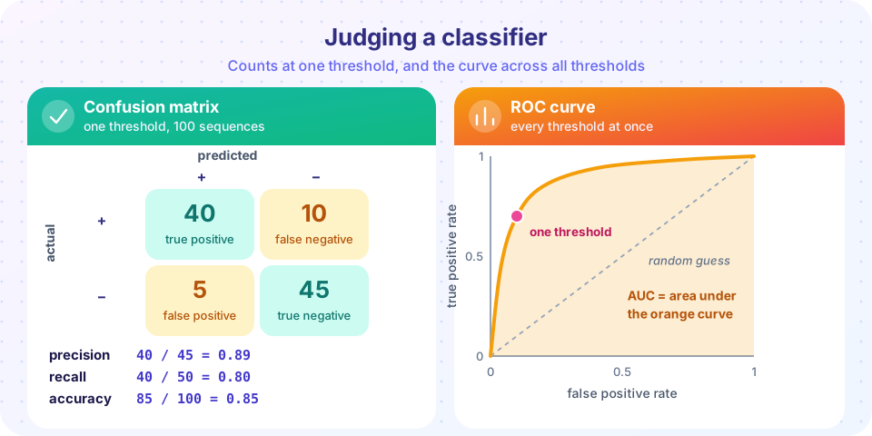
A classifier usually outputs a score (a probability); you choose a threshold and call everything above it positive. At that threshold you can count four outcomes, as in the figure: 40 true positives, 10 false negatives (missed positives), 5 false positives (false alarms) and 45 true negatives. From these:
| Metric | Formula | Example |
|---|---|---|
| Accuracy | (TP + TN) / total |
85 / 100 = 0.85 |
| Precision (positive predictive value) | TP / (TP + FP) |
40 / 45 = 0.89 |
| Recall (sensitivity, true positive rate) | TP / (TP + FN) |
40 / 50 = 0.80 |
| Specificity (true negative rate) | TN / (TN + FP) |
45 / 50 = 0.90 |
| False positive rate | FP / (FP + TN) |
5 / 50 = 0.10 |
| F1 score | 2 * precision * recall / (precision + recall) |
about 0.84 |
Raising the threshold makes the model more cautious: fewer false positives but more misses. Lowering it does the opposite. There is no free lunch, only a trade-off that you choose according to the cost of each error. A screening test wants high recall (do not miss cases), while a test that triggers an expensive follow-up experiment wants high precision.
Why accuracy fails for rare positives
Imagine 10,000 candidate variants of which 100 (1%) are truly damaging. A lazy classifier that says "benign" every time scores 99% accuracy and finds none of them. A real classifier that catches 80 of the 100 but also flags 400 benign ones has accuracy 95.8%, lower than the lazy one, but it is far more useful. Its recall is 0.80 and its precision is 80 / 480, about 0.17. The numbers that matter here are recall and precision, which you should always report with the class balance. The Matthews correlation coefficient (MCC), (TP * TN - FP * FN) / sqrt((TP + FP)(TP + FN)(TN + FP)(TN + FN)), is another single number that stays honest under imbalance.
ROC curves and AUC
The ROC curve (receiver operating characteristic) sweeps the threshold from high to low and plots the true positive rate against the false positive rate. A perfect classifier hugs the top-left corner; a useless one follows the diagonal. The AUC has a neat meaning: it is the probability that a randomly chosen positive example gets a higher score than a randomly chosen negative one. An AUC of 0.5 is chance, 1.0 is perfect. It is computed from ranks, so it does not depend on any one threshold and is insensitive to the class ratio.
That insensitivity is also a weakness when positives are rare. With 100 positives among 10,000, a false positive rate of 5% means 495 false alarms, enough to bury 80 true hits (precision under 15%). Yet that operating point looks excellent on the ROC curve, because the rate is computed over the huge negative class.
Precision-recall curves
The precision-recall (PR) curve plots precision against recall as the threshold sweeps. It focuses entirely on the positives and the cost of false alarms relative to them. A random classifier's PR curve is a horizontal line at the fraction of positives (1% in the example), so the baseline is not 0.5. The summary number is the average precision (area under the PR curve). For rare-positive problems such as finding variants, binding sites or pathogenic mutations, the PR curve is usually the more informative picture; for balanced problems the two agree closely.
Splitting data honestly
A model must be tested on data it never saw. The standard design is train / validation / test: fit on the training set, tune choices (features, regularization) on the validation set, and touch the test set once, at the end. With small data, use k-fold cross-validation: split into k parts, train on k-1 and test on the remaining one, rotate, and average. Stratified folds keep the class ratio in each part.
Leakage
Data leakage means information from the test set reaching training, directly or indirectly. In biology the sneakiest form is homology: if your set contains a protein and 20 of its close relatives, a random split puts some in training and some in testing. The model can score highly by recognizing "this looks like something I memorized", without learning any general rule. Other leaks include:
- exact or near-duplicate sequences, which databases often contain;
- features computed from the whole dataset before splitting (for example selecting the best genes using all samples);
- repeated measurements from the same patient or the same cell line in both sets;
- information about the label hidden in file names, batch or source.
The cure is group-aware splitting. Cluster sequences by similarity (tools such as CD-HIT or MMseqs2 cluster proteins at a chosen identity like 30%), assign whole clusters or whole gene families to one side, or hold out entire chromosomes or species. The harder the split, the more honest the score, and the lower it usually is. Bootstrap or repeated-split confidence intervals show how much the number could move by chance, which matters when the test set has few positives.
Finally, always compare against baselines (a threshold on one feature, or a nearest-neighbor model) and against a model trained on shuffled labels. If the shuffled-label model scores above chance, you have a leak.
Common misconceptions
"AUC 0.95 means 95% accuracy." AUC is a ranking quality, not an accuracy. It says nothing about calibration or the best threshold, and it can look excellent when precision is poor.
"A high cross-validation score proves the model generalizes." Only if the folds are independent. With related sequences in random folds, cross-validation can be wildly optimistic.
"I tuned on the test set a few times, but only lightly." Every peek makes the test score optimistic. Keep a final test set untouched.
Try it
First, compute metrics for a balanced and an imbalanced situation. Second, draw ROC and precision-recall curves for the same classifier at two class ratios. Third, run the leakage experiment: labels that are pure noise, yet a random split appears to find a pattern.
Press Run (or Ctrl + Enter) to see the result here.
Program input · what you'd type while the program runs
Type the answers before you press Run, one per line. Each time the program reads a line (with input()), it gets the next line from this box.
Press Run (or Ctrl + Enter) to see the result here.
Program input · what you'd type while the program runs
Type the answers before you press Run, one per line. Each time the program reads a line (with input()), it gets the next line from this box.
Press Run (or Ctrl + Enter) to see the result here.
Program input · what you'd type while the program runs
Type the answers before you press Run, one per line. Each time the program reads a line (with input()), it gets the next line from this box.
Check your understanding
Quick check · 5 questions
of 5 answered You scored / 5 · perfect!
-
1. A model finds 30 of 40 true binding sites and also flags 10 sequences that are not sites. What is its precision?
TP = 30 and FP = 10, so precision = 30 / 40 = 0.75 (recall is 30 / 40 as well). -
2. Only 0.5% of examples are positive. Which metric is the most misleading to report alone?
A model that always predicts negative has 99.5% accuracy but finds no positives. -
3. What does an AUC of 0.5 mean?
AUC is the probability that a random positive outscores a random negative; 0.5 is guessing. -
4. Which split best guards against homology leakage for a protein dataset?
Keeping relatives on the same side prevents the model from scoring by recognizing near copies. -
5. Which is a good test for a hidden leak?
A model with no real signal must score at chance on shuffled labels; anything higher indicates leakage or a bug.
Summary
- A threshold turns scores into a confusion matrix (TP, FP, FN, TN); precision, recall, specificity and F1 are ratios of its cells.
- Accuracy deceives when positives are rare; report precision and recall (or MCC) with the class balance.
- ROC curves and AUC (the probability that a random positive outranks a random negative) summarize all thresholds; PR curves and average precision are more informative for rare positives.
- Use train/validation/test splits or cross-validation, and group related sequences (families, clusters, chromosomes) so nothing leaks.
- Check with baselines and shuffled labels, and report confidence intervals.
Track your progress
Create a free account to tick off lessons and pick up where you left off on any device.
of Bioinformatics lessons completed