


















Lesson 21 of 49 · Phylogenetics
Parsimony and maximum likelihood
Learn character-based tree building: Fitch parsimony counting, long-branch attraction, likelihood under the Jukes-Cantor model, rate variation, model selection and Bayesian methods.
Distance methods squeeze an alignment into a single table of numbers, discarding which sites differed and how. Character-based methods keep the alignment column by column and ask, for every candidate tree, how well it explains each column. Two ideas dominate. Maximum parsimony prefers the tree that needs the fewest evolutionary changes. Maximum likelihood prefers the tree that makes the observed alignment most probable under an explicit model of evolution. A third family, Bayesian inference, builds on likelihood and returns a probability distribution over trees. These methods are slower than neighbor-joining but are the standard for careful work.
What you will learn
- Fitch's algorithm for counting changes on a given tree, and which sites are informative.
- Why parsimony can fail (long-branch attraction).
- How likelihood works, with the Jukes-Cantor transition probabilities and a two-sequence example.
- Rate variation among sites, model selection with AIC and BIC, and what Bayesian methods add.
Key terms
- Parsimony score: the minimum number of changes a tree needs to explain the alignment.
- Informative site: a column that can distinguish between trees (at least two states, each in at least two sequences).
- Likelihood: the probability of the data given a tree, branch lengths and a substitution model.
- Substitution model: rules (rates and base frequencies) describing how states change over time.
- Posterior probability: the probability of a tree or clade given the data, the model and a prior.
Maximum parsimony and Fitch's algorithm
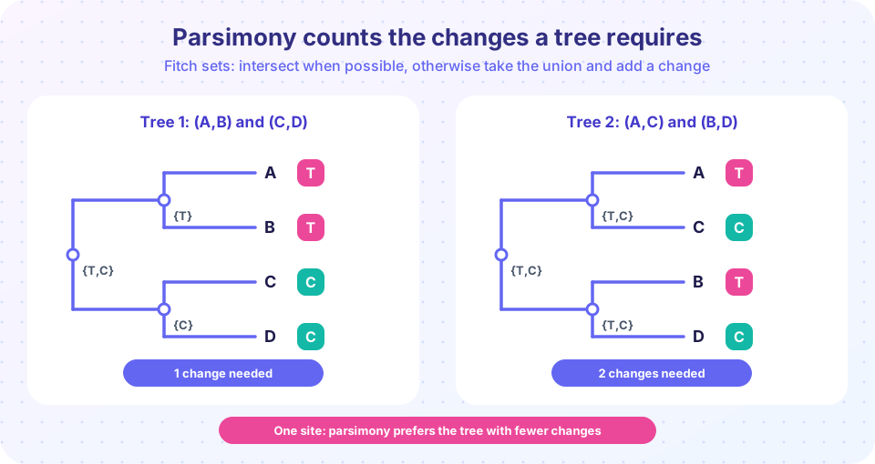
Parsimony applies Occam's razor: the best tree explains the data with the fewest changes. For one alignment column and one tree, the minimum number of changes is found by Fitch's algorithm (1971). Go from the leaves toward the root. Each leaf has the set containing its own state. For an internal node, intersect the sets of its two children. If the intersection is not empty, use it. If it is empty, take the union and count one change. The total of changes over the whole tree is the column's cost, and summing over columns gives the tree's parsimony score.
On the picture's example, the leaves A and B have T and C and D have C. On the tree that joins A with B and C with D, the (A,B) node gets {T}, the (C,D) node gets {C}, and the root's children do not overlap, so the root is {T,C} and one change is counted. On the tree that joins A with C and B with D, each of the two internal nodes would need {T,C} (two changes). With many columns, the tree with the lowest total wins.
Only informative sites matter. A column that is the same in every sequence, or that differs in only one sequence (a singleton), costs the same on every tree and cannot discriminate between them.
Finding the best tree is the hard part. Fitch's algorithm scores a tree; to find the best tree you must search. Small problems use exhaustive or branch-and-bound searches. Larger ones use heuristics that start with a tree and rearrange it (nearest-neighbor interchange, subtree pruning and regrafting) while the score improves.
Parsimony ignores branch lengths and assumes that change is rare. Its famous failure, described by Joseph Felsenstein in 1978, is long-branch attraction: two lineages that evolve fast accumulate many changes, some of which coincide by chance, and parsimony groups them together as relatives even when they are not. The effect gets worse with more data, because the method is consistently misled. Likelihood methods with a good model are less susceptible.
Maximum likelihood
Likelihood asks a different question: given a tree T with branch lengths, and a model M, what is the probability of observing the alignment? We choose the tree and branch lengths that maximize it.
The simplest model is Jukes-Cantor. If a site is observed after t expected substitutions per site, the probability that it still shows the original base is P_same(t) = 1/4 + (3/4) e^(-4t/3), and the probability that it shows one specific different base is P_diff(t) = 1/4 - (1/4) e^(-4t/3). As t grows, both approach 1/4, which is saturation again.
For two sequences with n sites, of which k differ, the likelihood of a distance d is, treating sites as independent and the root as the midpoint,
L(d) = (1/4)^n * P_same(d)^(n - k) * P_diff(d)^k
Maximizing this over d gives exactly the Jukes-Cantor distance d = -(3/4) ln(1 - 4p/3) with p = k/n. So the correction from the previous lesson is simply the maximum-likelihood estimate under that model.
For a tree with many leaves, the likelihood of one site sums over all possible states at the unobserved internal nodes. Felsenstein's pruning algorithm (1981) does this efficiently by working from leaves to root and reusing partial results. The likelihood of the whole alignment multiplies across sites, so programs add log-likelihoods instead. Programs then optimize branch lengths for each candidate tree and search the space of trees with rearrangement moves.
Better models: rates, frequencies and model choice
JC assumes equal base frequencies and equal rates among all substitutions. Real data show transition/transversion bias and unequal base frequencies, so richer models are used: K80 (a transition/transversion ratio), HKY (adds base frequencies) and GTR (general time-reversible, six exchange rates and four frequencies). Sites also evolve at different speeds: a third codon position changes more than a first or second. This is handled with +G, a gamma distribution of rates among sites with shape parameter alpha, and +I, a fraction of invariant sites. Protein trees use empirical matrices such as LG or WAG.
Choosing among models is itself a statistical task. More parameters fit better but may overfit. The Akaike information criterion AIC = 2k - 2 ln L and the Bayesian information criterion BIC = k ln(n) - 2 ln L, where k is the number of free parameters and n the number of sites, penalize complexity; the lowest value wins. Programs such as ModelFinder (in IQ-TREE) and ModelTest-NG do this automatically. Common maximum likelihood programs are IQ-TREE, RAxML-NG, PhyML and, for very large data sets with an approximate likelihood, FastTree.
Bayesian inference
Bayesian programs such as MrBayes and BEAST combine the likelihood with prior beliefs and return a posterior distribution of trees, usually sampled by Markov chain Monte Carlo. The posterior probability of a clade is the fraction of sampled trees that contain it. BEAST adds relaxed molecular clocks and calibration dates, so it can estimate when lineages split, which is how viral outbreaks are dated. Bayesian methods are the most computationally demanding, and you must check that the chains have converged.
Choosing among methods
| Method | Strength | Weakness |
|---|---|---|
| Neighbor-joining | Very fast, good first look | Uses only distances |
| Parsimony | No model needed, easy to explain | Long-branch attraction; ignores branch lengths |
| Maximum likelihood | Model-based, usually accurate | Slower; depends on model fit |
| Bayesian | Gives probabilities; supports dating | Slowest; needs priors and convergence checks |
Common misconceptions
- "Parsimony is model-free." It makes assumptions (change is rare and equally likely along branches), which fail with fast evolution.
- "More sites always fix a wrong method." For long-branch attraction, more data make parsimony more confidently wrong.
- "The likelihood is the probability that the tree is correct." It is the probability of the data given the tree; the tree's probability needs a prior (Bayesian analysis).
- "A more complex model is always better." Use AIC or BIC to balance fit and complexity.
Try it
Press Run (or Ctrl + Enter) to see the result here.
Program input · what you'd type while the program runs
Type the answers before you press Run, one per line. Each time the program reads a line (with input()), it gets the next line from this box.
Press Run (or Ctrl + Enter) to see the result here.
Program input · what you'd type while the program runs
Type the answers before you press Run, one per line. Each time the program reads a line (with input()), it gets the next line from this box.
Check your understanding
Quick check · 6 questions
of 6 answered You scored / 6 · perfect!
-
1. In Fitch's algorithm, what happens when the state sets of two child nodes do not overlap?
An empty intersection means at least one change; the parent set becomes the union. -
2. Which column is parsimony-informative?
At least two states must each occur in two or more sequences (A A G G). -
3. What is long-branch attraction?
Chance similarities on long branches are misread as shared ancestry, particularly by parsimony. -
4. For two sequences with p = 0.2, what does the Jukes-Cantor maximum-likelihood distance equal?
d = -0.75 ln(1 - 4(0.2)/3) = 0.233. -
5. Which criterion prefers the lowest value, penalizing the number of parameters?
AIC and BIC balance goodness of fit against model complexity. -
6. What does a Bayesian analysis add compared with maximum likelihood?
Bayesian methods combine the likelihood with priors to give posterior probabilities.
Summary
- Parsimony counts changes with Fitch's algorithm and prefers the tree that needs the fewest; only informative sites matter.
- Likelihood scores a tree by the probability of the alignment under a substitution model; the JC distance is its simplest maximum-likelihood estimate.
- Use richer models (GTR, +G, +I) chosen by AIC or BIC; Bayesian methods add priors and posterior probabilities.
- Parsimony can be misled by long branches; likelihood with a good model is more robust.
Track your progress
Create a free account to tick off lessons and pick up where you left off on any device.
of Bioinformatics lessons completed