


















Lesson 45 of 49 · Projects and Practice
Project: Differential Expression from Scratch
Simulate an RNA-seq experiment, normalize counts, test every gene, control the false discovery rate, draw volcano and MA plots, and measure how replicates affect power.
The RNA-seq lessons explained each idea separately: normalization, testing, multiple-testing correction, plots. In this project you put them together in one script and, as in the variant-calling project, you will know the truth. You will simulate an experiment in which 100 of 1,000 genes really change, run a complete analysis, and measure how many true changes it finds and how many false ones it reports.
Knowing the truth lets you answer a question that real experiments cannot: how much do replicates matter? You will end with a power curve that shows what happens to your ability to detect real changes as the number of biological replicates grows from two to twelve.
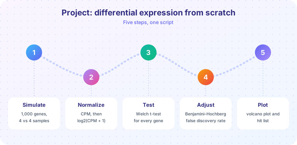
What you will build
- A simulator that draws gene counts from a negative binomial model with different library sizes and 100 truly changed genes.
- A normalization step using median-of-ratios size factors and a log2 transform.
- A per-gene Welch t-test on log values, with Benjamini-Hochberg adjustment.
- A hit list and an evaluation against the truth.
- Volcano and MA plots.
- A power analysis over the number of replicates.
Key terms
Negative binomial counts: Poisson counts whose rate varies between replicates; here made by drawing a Gamma rate, then a Poisson count.
Size factor: a per-sample scaling number; the median-of-ratios method estimates it.
Power: the probability of detecting a gene that is truly changed.
Realized FDR: the fraction of your called genes that are truly unchanged, computable only in simulation.
MA plot: log fold change against mean expression.
Step 1: simulate and test
The simulator gives each gene a base expression drawn from a log-normal distribution (a few genes are highly expressed, most are modest). One hundred randomly chosen genes get a true log2 fold change of magnitude between 1 and 2.5, up or down. Each sample gets a library-size factor between 0.7 and 1.4, so normalization has real work to do. The expected count of gene g in sample s is mu = base * 2^lfc * depth_s for treated samples and base * depth_s for controls. Counts are then drawn with a dispersion of 0.1, matching the typical biological variation of about 30% described in the differential-expression lesson.
The analysis follows the lessons: compute size factors by median-of-ratios, normalize, transform with log2(x + 1), run a Welch t-test for each gene (which does not assume equal variances), and adjust p-values with Benjamini-Hochberg. A t-test on log values is a simple stand-in for the negative binomial tests in DESeq2 or edgeR, and it works acceptably when replicates are not too few and counts are not tiny. Run the full pipeline and look at the hit list.
Press Run (or Ctrl + Enter) to see the result here.
Program input · what you'd type while the program runs
Type the answers before you press Run, one per line. Each time the program reads a line (with input()), it gets the next line from this box.
Step 2: look at the result
A hit list is hard to judge, so draw the standard plots. The volcano plot shows log2 fold change against -log10(p); the true changed genes should sit in the upper left and right. The MA plot shows the log fold change against the mean expression; with good normalization, the bulk of unchanged genes forms a horizontal cloud centered on zero, and low-count genes scatter more widely. If the cloud sits above or below zero, the normalization failed.
Press Run (or Ctrl + Enter) to see the result here.
Program input · what you'd type while the program runs
Type the answers before you press Run, one per line. Each time the program reads a line (with input()), it gets the next line from this box.
Step 3: how many replicates do you need?
The final question is the one an experimental biologist asks before starting: with a fixed effect size and fixed variability, what do I gain from each additional replicate? In this script, we repeat the whole experiment for different numbers of replicates per group, five random seeds each, and measure power and the realized false discovery rate.
Press Run (or Ctrl + Enter) to see the result here.
Program input · what you'd type while the program runs
Type the answers before you press Run, one per line. Each time the program reads a line (with input()), it gets the next line from this box.
Reading the results
Two things should stand out. First, power rises steeply with replicates: with two or three per group this simple t-test finds essentially nothing, because variance estimates from so few samples are unstable and no p-value can get small enough to survive correction for 1,000 tests. With four per group it finds a good fraction of the large changes, with six it finds most, and by twelve it finds nearly everything whose effect is at least a two-fold change. (DESeq2 and edgeR do better at three replicates than this plain t-test because they borrow information about variability across genes, which is exactly why they exist.) Second, the realized FDR hovers near its target of 5% but need not equal it. The BH procedure controls the expected proportion of false discoveries under its assumptions; a t-test on small samples with skewed data is only an approximation, so treat the realized FDR as a diagnostic, not a guarantee.
Compare this with the real world. Actual experiments have more variability than this simulation, effect sizes are often smaller than a two-fold change, and some replicates fail quality control. That is why experienced analysts plan for more replicates than the bare minimum, and why a published list of "significant genes" from a three-versus-three experiment should be read as a list of strong candidates, not as the full set of affected genes.
Why each analysis choice was made
Why a log transform? Counts have a variance that grows with the mean, so a gene with 10,000 reads would dominate any comparison on the raw scale. Taking log2(x + 1) makes variation roughly proportional across genes and turns fold changes into differences, which a t-test can handle. The added 1 avoids taking the logarithm of zero, at the cost of slightly distorting very low counts.
Why size factors instead of total counts? The two give similar answers when most genes do not change, but total-count scaling is vulnerable to a few strongly changed genes, as the normalization lesson showed. With 10% of genes changed in both directions the difference is small here; in an experiment where a few genes absorb a large share of reads it can be large.
Why Benjamini-Hochberg? With 1,000 tests and no correction, a 5% threshold would produce around 45 false positives among the 900 unchanged genes. Controlling the false discovery rate keeps the list trustworthy while still finding many real changes, unlike a Bonferroni threshold that would find fewer.
Why a fixed fold-change threshold is not applied. The hit list uses only the adjusted p-value. Many studies also require |log2FC| > 1, which removes statistically significant but biologically tiny changes. Try adding that filter and watch the number of hits and the false discoveries change; this is the effect-size-versus-evidence trade-off from the differential-expression lesson in action.
Extensions to try
- Raise the dispersion from 0.1 to 0.4 and re-run the power curve; how many more replicates compensate?
- Shrink the effect sizes so true changes have |log2FC| between 0.3 and 1, and see how power collapses.
- Break the normalization: skip the size factors and divide only by total counts after adding one very highly expressed gene that changes strongly; what happens to the MA plot?
- Add a batch effect: add a shift to half the samples in each group and see how a plain t-test fares compared with one that includes batch as a covariate (for instance with a regression).
- Replace the t-test with a likelihood-ratio or Wald test on a negative binomial fit using
statsmodelsand compare the number of hits.
Check your understanding
Quick check · 5 questions
of 5 answered You scored / 5 · perfect!
-
1. Why are different library-size factors included in the simulation?
Real samples are sequenced to different depths; the size factors must correct this. -
2. Which statement about the Welch t-test is correct?
Welch's version of the t-test allows unequal variances, which is safer for expression data. -
3. In an MA plot after good normalization, the cloud of unchanged genes should be centred on:
Most genes are unchanged, so their log fold changes should centre on zero. -
4. What is the main reason power is low with two replicates per group?
With so few samples, variance is poorly estimated and the evidence cannot reach significance after correction. -
5. A 'realized FDR' can be computed only in simulation because:
In real data the truth is unknown, so the false discoveries cannot be counted directly.
Summary
- A simulation with known truth lets you grade a complete analysis: power, false discoveries and the effect of design choices.
- The pipeline: negative binomial counts, median-of-ratios size factors, log2 transform, Welch t-test per gene, BH adjustment, volcano and MA plots.
- Replicates, not depth, drive power; with two per group, most real changes are missed.
- Treat realized FDR as a diagnostic: approximate tests and small samples can drift from the nominal 5%.
Next: Practice Problems
Track your progress
Create a free account to tick off lessons and pick up where you left off on any device.
of Bioinformatics lessons completed